
Karteikarten
Flashcards Terms
Karten in diesem Stapel (72)
- 1Layer NormalizationThe Layer Normalization operation is a method to standardize the inputs to a layer for each mini-batch, i.e., it ensures that the inputs have a mean of 0 and variance of 1. The 'LayerNorm.weight' and 'LayerNorm.bias' are learnable parameters that shift and scale this standardized output, respectively.
- 2Bias termsThe bias term allows the activation function to be shifted to the left or the right, to better fit the data.
- 3Weight decayWeight decay is a form of regularization, which is a technique used to prevent overfitting.
Weight decay specifically is a method of regularization that discourages large weights in the model by adding a penalty proportional to the size of the weights. It works by adding a term to the loss function that is proportional to the square of the magnitude of the weights. This encourages the model to keep the weights as small as possible, which in turn encourages the model to be as simple as possible. Simpler models are less likely to overfit, as they have less capacity to memorize the training data. - 4OverfittingOverfitting occurs when a model learns the training data too well, to the point that it performs poorly on unseen data because it has essentially memorized the training data instead of learning the general patterns. Regularization addresses this issue by adding a penalty to the loss function that increases with the complexity of the model.
- 5model.named_parameters()model.named_parameters() is a PyTorch method that returns an iterator yielding the names (string) of all the parameters of a model and the parameters themselves. When we cast this to a list, we get a list of tuples, where each tuple is a pair consisting of the name of the parameter as a string and the parameter itself.
The parameters of a model are the elements that are learned during the training process to minimize the loss function. In the case of a neural network, these parameters are the weights and biases of the network. - 6cache directorya cache directory is a location on disk where the pretrained models will be stored after they're downloaded.
When you use a method like BertForSequenceLabeling.from_pretrained, it needs to load the weights of a pre-trained BERT model. The first time you run this, it will download the weights from the internet, which can take a bit of time depending on the size of the model and your internet connection.
To avoid downloading the model every time you run your script, the weights are stored ("cached") on your local disk after the first download. The next time you run your script, the method will see that the weights are already available in the cache directory and load them from there, which is much faster than downloading them from the internet. - 7fp16The --fp16 argument is used to enable mixed-precision training. Typically, the weights and activations in a neural network are stored as 32-bit floating point numbers (also known as float32 or fp32). However, modern GPUs can also work with 16-bit floating point numbers (float16 or fp16), which require less memory and allow the model to run faster.
Mixed-precision training means that some of the weights and activations are stored as fp16 to take advantage of these benefits, while others are kept as fp32 to avoid issues with numerical precision. The --fp16 argument is a flag that enables this mode. - 8loss scaleThe --loss_scale argument is related to this. When working with fp16 numbers, one issue that can arise is underflow: if a number is very small, it might be rounded down to zero in fp16 format. To prevent this, the gradients (which can be quite small numbers) are typically scaled up by a large factor before being applied. After the weight update, the weights are scaled back down again. This process is known as loss scaling.
The --loss_scale argument specifies the factor to use for this process. If it's set to 0 (the default), dynamic loss scaling is used, which means that the scale factor is adjusted automatically based on the range of gradient values. If it's set to a positive power of 2, that value is used as a static loss scale factor. - 9seedThe --seed argument sets the initial seed for generating random numbers. This seed is used to initialize the random number generator in Python, NumPy, and PyTorch, which in turn affects many operations in machine learning, like weight initialization and shuffling of the data.
Setting a specific seed (42 in this case) ensures that the random processes in the script are deterministic. In other words, when you run the script multiple times with the same seed, you will get the same results. This is crucial for debugging, and for comparing the results of different algorithms or parameters: if you get a better result after changing something, you want to be sure it's because of your change, and not just due to a lucky set of random numbers. - 10learning ratethe learning rate for the Adam optimizer. The learning rate is a hyperparameter that determines the step size at each iteration while moving toward a minimum of a loss function.
In other words, when we train a model, we're trying to find the set of weights that minimize the difference between our predictions and the true values (this difference is quantified by the loss function). We do this by iteratively adjusting the weights in the direction that most decreases the loss function. The learning rate determines how much we adjust the weights at each step.
Often, the learning rate is set to start at a higher value and then gradually decrease. This strategy is called learning rate decay or scheduling. It's helpful because early in the training process, when the weights are likely far from their optimal values, larger steps can be taken without the risk of overshooting the minimum. - 11learning rate too small or too largeIf the learning rate is too large, the weights are adjusted too much at each step, and the optimization process may overshoot the true minimum and never converge (it may just keep bouncing around the minimum).
If it's too small, the weights are adjusted by a very small amount at each step, and the optimization process could take very long to converge. It could also get stuck in a local minimum rather than finding the global minimum. - 12gradient accumulation stepsThe --gradient_accumulation_steps argument is used in scenarios where your model is too large to fit in your GPU memory with your desired batch size.
This argument specifies how many forward passes (steps) the model should perform before doing a backward pass (updating the model weights).
For instance, if you set --gradient_accumulation_steps to 4, then the model will do 4 forward passes, each with (total batch size / 4) number of examples, and then do a backward pass.
This effectively allows you to work with a larger batch size than you could normally fit in memory, which can be beneficial for the training of certain models. This can be seen as a way to mimic a larger batch size while using less GPU memory. - 13warmupThe concept of "warmup" is often used in the context of learning rate scheduling in the training of deep learning models. During the warmup period, the learning rate gradually increases from a small value to a larger value. This strategy can help the model converge more stably and avoid drastic changes in parameter updates at the beginning of the training. After the warmup period, the learning rate usually starts to decrease.
- 14GRACE: Cascaded LabelingThis is a mechanism where the model labels the aspect terms first (using Aspect Term Extraction or ATE) and then uses these labels as part of the input to label the sentiment (using Aspect Sentiment Classification or ASC). This approach allows the model to take into account the interactions between aspect terms and their sentiment labels, which can improve performance.
- 15GRACE: Gradient Harmonized Loss (GHL)This is a technique used to adjust the model's loss function based on the frequency of different labels in the training data. The idea is that labels that are more common are usually easier for the model to predict, so GHL reduces the loss for these labels and increases the loss for less common (harder to predict) labels. This makes the model pay more attention to the less common labels during training.
- 16GRACE: Virtual Adversarial Training (VAT)This is a regularization method where the model is trained to be robust to small perturbations in the input data. The perturbations are chosen to increase the divergence between the model's predictions for the original and perturbed inputs. The goal is to make the model more robust and improve its generalization performance.
- 17Grid Search CVIn the context of machine learning and the Scikit-Learn library, "grid search CV" refers to "Grid Search Cross-Validation." It is a technique used for hyperparameter tuning, which is the process of finding the best set of hyperparameters for a machine learning model that yields the highest performance.
Grid search CV automates the process of hyperparameter tuning by searching through a specified set of hyperparameter values in a grid-like manner. It exhaustively tries all possible combinations of hyperparameters from the provided grid and evaluates the model's performance using cross-validation. - 18BoWThe following models a text document using bag-of-words. Here are two simple text documents:
(1) John likes to watch movies. Mary likes movies too.
(2) Mary also likes to watch football games.
Based on these two text documents, a list is constructed as follows for each document.
Representing each bag-of-words as a JSON object, and attributing to the respective JavaScript variable:
BoW1 = {"John":1,"likes":2,"to":1,"watch":1,"movies":2,"Mary":1,"too":1};
BoW2 = {"Mary":1,"also":1,"likes":1,"to":1,"watch":1,"football":1,"games":1};
Each key is the word, and each value is the number of occurrences of that word in the given text document.
The order of elements is free.
It is also what we expect from a strict JSON object representation.
Note: if another document is like a union of these two,
(3) John likes to watch movies. Mary likes movies too. Mary also likes to watch football games.
its JavaScript representation will be:
BoW3 = {"John":1,"likes":3,"to":2,"watch":2,"movies":2,"Mary":2,"too":1,"also":1,"football":1,"games":1}; - 19Adam OptimizerAdam, short for "Adaptive Moment Estimation," is a popular optimization algorithm used in deep learning models. It's an extension of stochastic gradient descent (SGD), the most fundamental optimization algorithm used to minimize a model's loss function.
Here are the key characteristics of the Adam optimizer:
Adaptive learning rates: Adam adjusts the learning rate for each parameter individually over time, based on the historical gradients. This is beneficial when dealing with complex neural networks where some parameters may require more adjustments than others.
Momentum: Adam maintains an exponentially decaying average of past gradients (also known as "momentum"). This helps the model to keep moving in the most promising direction rather than bouncing around randomly.
RMSprop: Adam also incorporates elements of another algorithm called RMSprop, which uses an exponentially decaying average of past squared gradients to adjust learning rates. This helps Adam deal with sparse gradients and makes it robust to noisy data. - 20FusedAdamThe FusedAdam optimizer is also a variant of the Adam optimizer optimized for NVIDIA's Apex library which can handle half-precision tensors.
- 21FP16_OptimizerFP16_Optimizer is a utility provided by the apex library, a PyTorch extension developed by NVIDIA for high performance computing. The purpose of the FP16_Optimizer is to handle Automatic Mixed Precision (AMP) training, which is a technique to improve the performance and reduce memory usage of deep learning models.
- 22OptimizersOptimizers in deep learning, such as Adam or Stochastic Gradient Descent (SGD), are algorithms used to change the attributes of your neural network such as weights and learning rate in order to reduce the losses. These algorithms play a key role in defining how changes to the model are made during training: they navigate the weight space using the gradient of the loss function with respect to the weights, computed via backpropagation.
Here's the general flow:
Forward pass: The model makes a prediction based on the current values of the parameters (weights and biases).
Loss calculation: The loss or error is calculated by comparing the model's prediction and the actual target.
Backward pass (Backpropagation): The gradients of the loss function with respect to the model's parameters are computed.
Optimization step: The optimizer updates the model's parameters (e.g., weights and biases) using their gradients to minimize the loss. - 23all_input_ids = torch.tensor([f.input_ids for f in features], dtype=torch.long)These lines are creating 2D tensors (you can think of these as similar to 2D arrays or tables). Each tensor corresponds to a particular feature that will be used as input to the model.
all_input_ids: This tensor contains the tokenized text inputs that will be fed into the model. Each row in the tensor corresponds to a different training example, and each column corresponds to a different token ID in that example. These IDs are how the model identifies the words: each unique word or sub-word is mapped to a unique ID. - 24convert_examples_to_features()The convert_examples_to_features() function processes each data item (often referred to as an "example" or "instance") individually, and outputs a list of "features". Each item in the list corresponds to one data item, like a sentence.
The function takes a sentence and processes it into a format suitable for the model. This involves tokenizing the text, converting the tokens into IDs (which the model can understand), creating segment IDs (if needed), and creating an attention mask.
These processed elements—input IDs, segment IDs, and the attention mask—are bundled together into a single object (usually a simple data structure like a Python class). This object represents the "features" extracted from the original text sentence.
The function repeats this process for each sentence in the dataset, and the resulting "features" objects are appended to a list. - 25Input IDIn the context of transformer-based models like BERT, an "input ID" refers to the specific numerical representation of a token (i.e., a word or sub-word) in the vocabulary of the transformer model.
The tokenization process breaks down the text into smaller pieces, which are called "tokens". In English, tokens can be as short as one character or as long as one word (e.g., "a", "apple"). They could also be subwords for languages or words that don't exist in the pre-trained model's vocabulary.
Each unique token in the model's vocabulary has a unique integer assigned to it, known as its "ID". So the "input IDs" are just the IDs corresponding to the tokens in the input sentence.
For example, if the vocabulary of the model is {"a": 0, "an": 1, "apple": 2}, the sentence "an apple" would be tokenized into ["an", "apple"], and the corresponding input IDs would be [1, 2]. - 26Segement ID"segment IDs" are used to differentiate different sentences in the same input. In some tasks, the model needs to take two sentences as input (e.g., question-answering, natural language inference). The "segment IDs" are used to distinguish the two sentences. Typically, all tokens from the first sentence will get a segment ID of 0, and all tokens from the second sentence will get a segment ID of 1. If there's only one sentence in the input, then all tokens will get a segment ID of 0.
- 27Tokenizer + VocabularyThe tokenization process is dependent on the specific tokenizer used, and the tokens' numerical representations (the "input IDs") are dependent on the model's vocabulary file.
In the vocabulary file of a pretrained model, each unique token is mapped to a unique ID. The tokenizer, which is usually trained together with the model, knows how to break down text into these tokens and how to map tokens to their respective IDs based on this vocabulary.
For instance, in the BERT model, a WordPiece tokenizer is used. This tokenizer can break words into smaller units (subwords or characters) if a word is not found in the vocabulary. For example, the word "unaffable" might be broken down into ["un", "##aff", "##able"] if "unaffable" itself is not in the vocabulary but "un", "##aff", and "##able" are.
The vocabulary file and the tokenizer must align. If you use the tokenizer from one model with the vocabulary from another, you won't get meaningful results. - 28TokenizerA tokenizer is a method that breaks down text (such as sentences) into smaller components, called tokens. These tokens can be as long as a word or as short as a character. The exact rules for what counts as a token depend on the tokenizer.
After tokenization, the tokenizer maps each token to a unique ID, as defined in a vocabulary file. These IDs are what the model actually processes. The vocabulary file is created during the pre-training phase and is specific to each language model. It contains a unique ID for each token the model knows.
So overall, a tokenizer serves two main functions:
1. Break down the text into tokens (tokenization).
2. Map each token to a unique ID (numerical representation) as per the vocabulary file. - 29all_input_mask = torch.tensor([f.input_mask for f in features], dtype=torch.long)This tensor indicates which elements in the input_ids tensor correspond to actual tokens versus padding. It's common to pad all sequences in a batch to the same length for computational efficiency. This mask allows the model to ignore the padding when computing the output.
- 30all_segment_ids = torch.tensor([f.segment_ids for f in features], dtype=torch.long)all_segment_ids: This tensor is used to distinguish different sentences in the same input. For example, in a pair of sentences, the first sentence would have segment_ids of 0, and the second would have segment_ids of 1. For single sentence tasks, this tensor will just be all zeros.
- 31TensorDatasetThis is a utility class provided by PyTorch that represents a dataset of tensors. Each tensor in the dataset corresponds to a different feature or label. In this case, all_input_ids, all_input_mask, all_segment_ids, and all_label_ids are all tensors, so you can use them to create a TensorDataset. When you iterate over a TensorDataset, it yields tuples where each element of the tuple corresponds to a different tensor in the dataset. For example, if you do for x in train_data, where train_data is a TensorDataset, x will be a tuple with four elements, where the first element is a sample of all_input_ids, the second is a sample of all_input_mask, and so on.
- 32RandomSamplerThis is another utility provided by PyTorch. It defines a way to iterate over the indices of a dataset. It does not directly interact with the data, but it provides an order to access them. In the case of RandomSampler, this order is random, meaning that each epoch the data will be accessed in a different order, adding an element of randomness to the training process which can help to improve the model's ability to generalize.
- 33DistributedSamplerThis is similar to RandomSampler, but it's designed for use in a distributed (multi-machine) training setting. The sampler will divide the dataset into a number of chunks equal to the number of machines, and each machine will then be assigned one chunk. This is useful for training on large datasets that may not fit into the memory of a single machine. If the script is not being run in a distributed environment, it uses the RandomSampler instead.
- 34DataLoaderA DataLoader in PyTorch is an iterator that provides a convenient way to iterate over a dataset. Its main functionality is to create batches of your data in an efficient way. It can take a Dataset (or a more traditional Python data structure like a list) and a Sampler, and combines them to allow easy iteration over your data in a way specified by the sampler.
The DataLoader object in PyTorch returns an iterator, so you can loop over it to get batches of data. Each item returned from the iterator is a batch, which is a tuple where the first element is a batch of inputs, and the second element is a batch of labels. The specific structure of the batches depends on how your dataset is structured. - 35SequentialSamplerInstead of the RandomSampler or DistributedSampler used during training, this function uses a SequentialSampler to iterate over the validation data in order. This is because during validation, the order of examples does not matter as we are not updating the weights of the model based on these examples.
- 36dropoutDropout is a regularization technique used in neural networks to prevent overfitting. Dropout works by randomly "dropping out" (i.e., setting to zero) a number of outputs from neurons in a layer during a forward pass. The idea is that this prevents neurons from relying too heavily on the outputs of the others, making them learn more robust and independent features. Dropout is only applied during training, and not during evaluation or testing.
- 37enumerate()In Python, enumerate() is a built-in function that allows you to loop over something and have an automatic counter. This counter is useful when you want to have the index of the item while you're iterating.
Here's a basic example:
for i, v in enumerate(['apple', 'banana', 'grapes']):
print(f"index: {i}, value: {v}")
This would output:
index: 0, value: apple
index: 1, value: banana
index: 2, value: grapes - 38"acc_sum"This likely represents the accumulated accuracy of the model's predictions. While it's not entirely clear without the implementation of the model, typically this would be the sum of correct predictions over the total number of predictions.
- 39"loss"This is the loss computed by the model given the inputs and the target labels. The loss is a scalar tensor (i.e., a tensor with a single value) that represents how well the model's predictions match the target labels. The goal of training is to minimize this loss.
- 40Cross EntropyIn a typical setup for a classification problem, a common loss function would be the Cross-Entropy loss. This loss function is used when the output of the model is a probability distribution over the classes (which is often the case in classification problems).
Cross-Entropy loss is calculated as the negative logarithm of the predicted probability for the true class. So if the model assigns a high probability to the correct class, the loss will be low, and if it assigns a low probability to the correct class, the loss will be high. - 41loss.backward()This line is calling the backward() function which is a built-in function provided by PyTorch's Autograd engine. The backward() function is used to compute the gradient of the loss with respect to the model parameters. These gradients are used during the optimization step to update the model parameters. If fp16 is not set to True, then standard backpropagation (float32) is used.
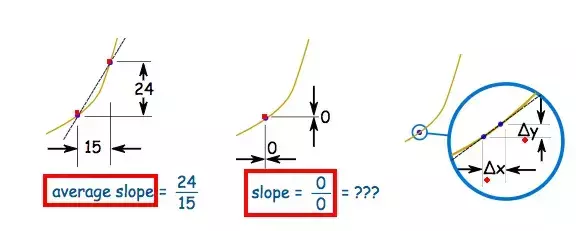
- 42Derivative of a functionThe derivative of a function at a certain point is essentially the slope of the function at that point. In other words, it represents how much the function changes if you make a tiny change in the input.
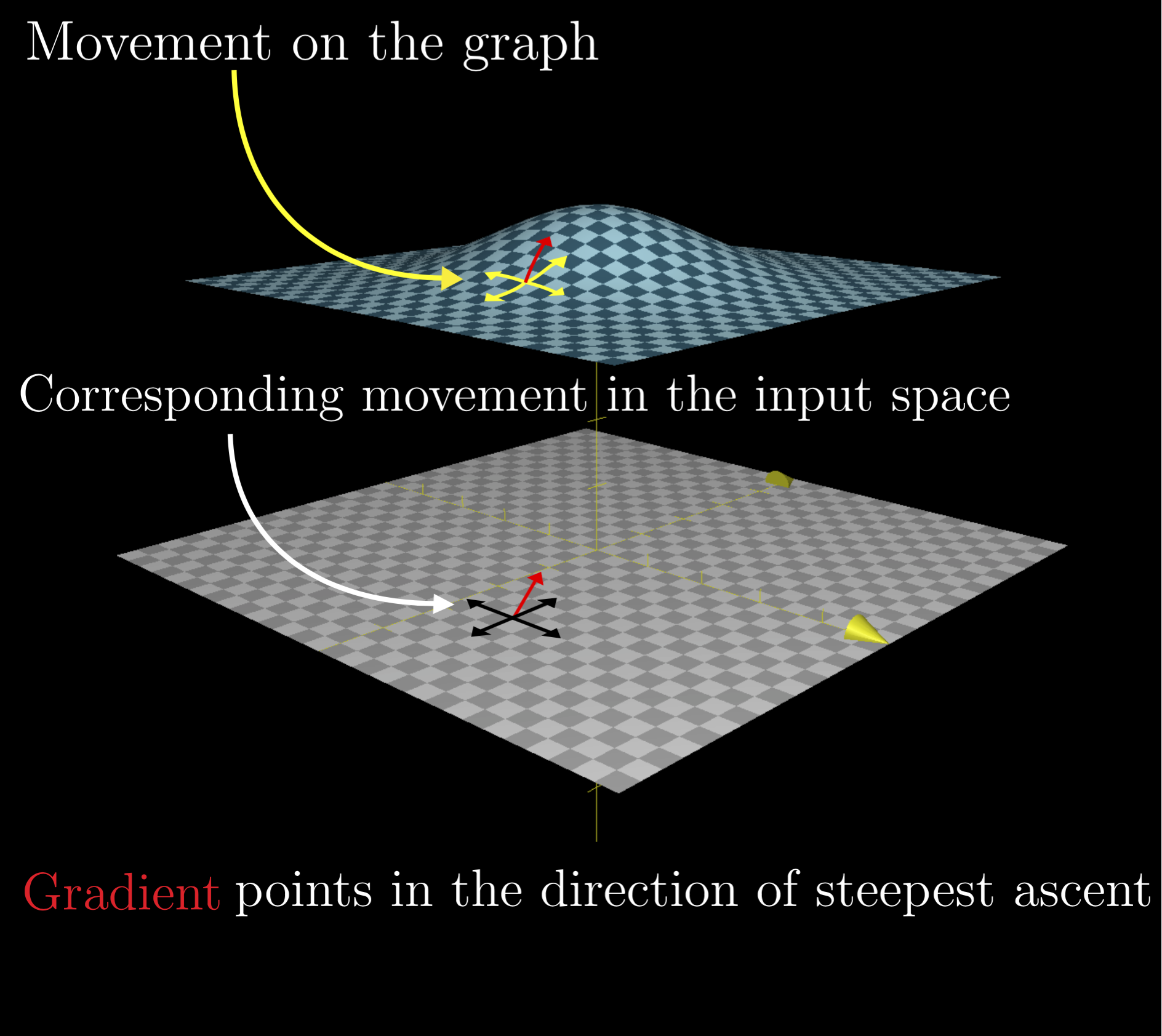
- 43gradientNow, when we move to functions of multiple variables (like a neural network, which has many weights), we can't talk about the derivative anymore because there isn't a single input. Instead, we talk about the gradient, which is a vector of partial derivatives. Each component of the gradient vector is the derivative of the function with respect to one weight, holding all the other weights constant. The gradient vector points in the direction in which the function increases the most.
- 44Gradient of the losswhen we say "gradient of the loss", we're talking about how much the loss function changes for small changes in each of the weights. If the gradient of the loss with respect to a weight is positive, it means that increasing that weight will increase the loss. Conversely, if it's negative, it means that increasing that weight will decrease the loss.
- 45optimizer.step()the optimizer's step() method is called to update the model's parameters
- 46optimizer.zero_grad()the optimizer's zero_grad() method is called to zero the gradients
- 47the benefit of a set over a listThe reason to convert the list into a set in this case is to utilize the properties of set operations to easily calculate quantities like the number of correct predictions and the total number of predictions.
Efficient membership tests: Checking whether an item is in a set is faster than checking whether it's in a list.
Easy set operations: Python sets have built-in methods to perform operations like intersection (common elements), union (all unique elements), difference (elements in one set but not the other), and symmetric difference (elements in either set, but not both). These operations are useful in various computation scenarios, including here where we are calculating precision, recall, and F1-score. - 48PrecisionPrecision (p) is the number of correct predictions divided by the total number of predictions.
Precision can be remembered as the measure of your model's "preciseness" or "exactness". In other words, how many of the items that your model identified as positive are actually positive. A mnemonic could be "Proper Positives". - 49RecallRecall (r) is the number of correct predictions divided by the total number of actual positive cases in the ground truth.
Recall, also known as sensitivity, can be remembered as the measure of your model's ability to identify all positive instances in the dataset. It tells you what portion of the actual positives was identified correctly. A mnemonic could be "Real Positives Recovered". - 50f1F1 score (f1) is the harmonic mean of precision and recall, and it gives you a single metric that looks at the balance between precision and recall. It's often used when you want to balance precision and recall and there isn't a clear preference between the two. This can be more useful than accuracy if the cost of false positives and false negatives are very different, or if the classes are imbalanced. A mnemonic could be "Fair Balance".
- 51accuracyAccuracy measures the proportion of total predictions (both positive and negative) that were correct. So it's an overall measure of how often the classifier is correct. A mnemonic could be "All Correct".
- 52when to use macro and micro f1 scoresthere are both macro and micro versions of F1 score, and they're used when you're working with datasets that have multiple classes, not just binary.
- 53Macro-F1This calculates the F1 score independently for each class and then takes the average. This treats all classes equally, regardless of their size, which might not be what you want if you have class imbalance.
if we compute a macro-F1, we average the precision and recall for each class and then use these averages to compute the F1 score. However, this method gives equal weight to both classes, even though class A has many more instances. - 54Micro-F1This aggregates the contributions of all classes to compute the average metric. In a multi-class classification setup, micro-F1 is preferable if you suspect there might be an imbalance among the classes.
The micro-F1 score gives you a single measure of how well your model is doing across all classes, with each instance in the dataset treated equally.
the micro-F1 score considers the total true positives, false negatives, and false positives over all classes:
Total true positives = 700 (for A) + 150 (for B) = 850
Total predictions = 800 (for A) + 200 (for B) = 1000
Total actual instances = 800 (for A) + 200 (for B) = 1000
So, the micro-averaged precision = micro-averaged recall = 850/1000 = 0.85, and thus, the micro-F1 score is 0.85. This gives us a single measure that considers the imbalance in the dataset. - 55logitsIn machine learning, the term "logits" refers to the unnormalized output of a model. These are the raw values that your model generates before it applies a normalization function like the softmax function. In the context of classification, these logits represent how likely each output class is according to the model. However, these values are not probabilities yet because they do not necessarily sum up to one and can be any real number.
it's not just a simple vector; rather, it's a tensor of shape (batch_size, sequence_length, num_labels).
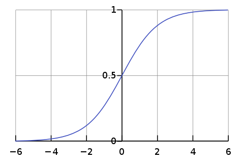
When you pass the inputs through the model, it will return a tensor, logits, of shape (batch_size, sequence_length, num_labels). So, if you're dealing with a batch of 32 sentences, each with a maximum length of 50 tokens, and your task is to classify each token into one of 3 possible classes, then your logits tensor will have a shape of (32, 50, 3). - 56Log-SoftmaxThe softmax function is used to convert logits into probabilities. It takes a vector of arbitrary real-valued scores (the logits) and squashes it to a probability distribution that sums to one. The log-softmax function is simply the logarithm of the softmax output. It's used because it's numerically more stable to deal with log probabilities, particularly to prevent underflow, which can occur when dealing with very small values.
- 57argmax()The argmax function does not return an ordered list but simply the index of the single highest value along a particular axis. In the code, argmax is used to select the class with the highest probability.
- 58logits.detach()Detachment from Computation Graph: When you perform computations in PyTorch, these operations are recorded to build up a computation graph. This graph is used during backpropagation to calculate gradients. When you "detach" a tensor, you remove it from the computation graph. After this point, no gradient will be backpropagated along this tensor, and the tensor's value won't be updated by gradient descent. In this case, the logits tensor is detached because we don't need to update the model (we're just evaluating it), and we want to prevent unnecessary computation.
- 59tqdm()tqdm is a Python library that allows you to output a smart progress bar by wrapping around any iterable. In this case, it's wrapping around the test data loader, so it will print a progress bar to the console that shows how many batches of the test data have been processed. This is particularly useful when you have a large test dataset and want to monitor the progress of the testing process.
- 60state_dict()The state_dict() function gets the model's parameters as a Python dictionary, which can then be saved to a file.
- 61GELU(x)GELU(x)=0.5x(1+erf(x/ √ 2))
GELU is believed to perform better in deeper architectures, like transformers, because it approximates the shape of a Gaussian distribution, which can be useful in handling the distribution of the inputs. This function helps the model during training and can lead to faster convergence in some cases.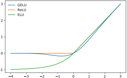
- 62swish(x)swish(x) = x * σ(x)
Why Swish?
The Swish activation function is a relatively newer activation function compared to others like ReLU, and it was introduced by researchers at Google. Swish tends to perform better than ReLU on deeper models across a range of tasks. It was found to be a more flexible function since it's bounded below (like ReLU) but unbounded above, and it has a non-monotonic nature (i.e., not always increasing or always decreasing). This property can help it adapt better during the training of deep networks. The activation is also smooth everywhere, which can help with gradient-based optimization.
In essence, Swish offers a balance of properties from both the ReLU and sigmoid functions, and has been found empirically to offer better performance in certain deep learning tasks.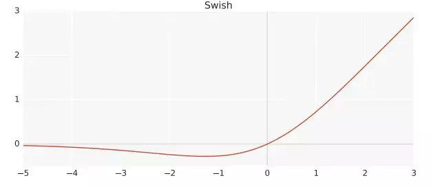
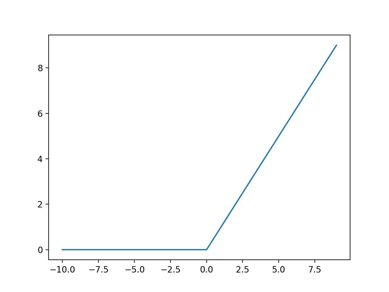
- 63ReLU(x)the ReLU (Rectified Linear Unit) activation function from PyTorch's functional module. It's one of the most commonly used activation functions in deep learning and is defined as f(x)=max(0,x).
- 64normalizationNormalization generally refers to the process of adjusting values measured on different scales to a common scale. In deep learning, normalization helps in stabilizing the training process and improves convergence.
- 65Batch NormalizationIntroduced in 2015 by S Ioffe and C Szegedy, batch normalization ("batch norm") normalizes across a batch of data.
How it works: For a given layer's output, batch norm computes the mean and variance for each feature across the mini-batch. These stats are then used to normalize the feature values across the mini-batch. So, for every feature, we use all the values of that feature across the batch to compute its mean and variance.
For a simple example, let's take a mini-batch of size 3 and a feature dimension of 2:
[[0.5, 1.0],
[0.6, 0.8],
[0.4, 1.2]]
For the first feature (across the batch), the mean is (0.5 + 0.6 + 0.4) / 3 = 0.5 and similarly, you'd compute the variance. Then, each value of the feature in the batch would be normalized using this mean and variance.
Why it helps: By normalizing the activations in the network, batch normalization reduces the amount by which the distribution of activations changes during training. This, in turn, mitigates the problem of internal covariate shift. - 66Layer (Feature) Normalization (BertLayerNorm)Layer normalization (or feature normalization) normalizes across the features, not across the examples in the batch.
How it works: For each individual data point in the mini-batch, layer normalization computes the mean and variance across its features and uses these statistics to normalize. So, each data point gets normalized by its own mean and variance.
Using the previous example:
[0.5, 1.0]
The mean is (0.5 + 1.0) / 2 = 0.75 and the variance is computed across these two features. The normalization is then done using this mean and variance for this particular data point.
Why it helps: Layer normalization helps in scenarios where batch size is small or dynamic (like in Recurrent Neural Networks). It's also invariant to batch size. - 67nn.Modulenn.Module is a fundamental class in PyTorch for building neural networks. It's a base class for all neural network modules, and encapsulates both the network layers and methods for manipulating the computations and parameters. Key points:
Parameter Management: nn.Module automatically keeps track of the params (weights and biases) of a network.
Customizable Forward Pass: By overriding the forward method, you can define the forward pass of your network/module.
Nesting: Instances of nn.Module can be nested so that an nn.Module can contain other nn.Modules, allowing for a hierarchical structure.
Device Agnostic: Modules can be moved across devices (e.g. CPU to GPU). Using methods like .to(), .cuda(), and .cpu(), you can move the entire module, incl. all parameters and buffers.
Built-in Methods:
.parameters(): Returns an iterator over the module's parameters.
.zero_grad(): Zeros out the gradient of all parameters.
.train() and .eval(): Switches to training or evaluation mode.
State Management: supports methods for saving, loading parameters, checkpointing and model persistence. - 68Weight Initialization with Ones (self.weight = nn.Parameter(torch.ones(hidden_size)))The weight parameter in the layer normalization represents a scaling factor. If you initialize it with ones, it means you're starting with the assumption that the normalized data doesn't need any scaling. During the training process, the model will adjust these weights as needed. If it was initialized with zeros, the output of the layer normalization would always be zero during the initial forward passes, which isn't desirable.
- 69Bias Initialization with Zeros (self.bias = nn.Parameters(torch.zeroes(hidden_size)))The bias parameter represents an additive offset. Initializing it with zeros means you're starting with the assumption that the normalized data doesn't need any bias adjustment. Again, during training, the model will adjust these bias values as required.
- 70Hidden size (or feature size)When dealing with sequences in models like BERT, the data often takes on a shape like:
batch size × sequence length × hidden size (or feature size)
Here's how you can interpret the statement "to calculate a mean across the feature dimension" in the context of this data shape:
Batch size: This dimension is the nr of sequences or samples you're processing simultaneously. Each "sample" might be a sentence.
Sequence length: This dimension is the nr of tokens in each sequence. For text, a token might be a word or subword.
Hidden size (or feature size): For each token in the sequence, the model will have a dense vector representation of a specific size (often called "hidden size" in the context of BERT). This representation captures various syntactic and semantic features of the token in its context. Each value or coordinate in this dense vector is essentially a "feature." - 71to calculate mean over feature dimensionwhen the BertLayerNorm class computes the mean across the last dimension (feature dimension), it does the following for each sequence in the batch:
For each token in the sequence, it averages its feature values. This gives you a single average value for each token.
In mathematical terms, given an output tensor x of shape [batch_size, sequence_length, hidden_size], the mean operation produces a tensor u of shape [batch_size, sequence_length, 1]. Each value in u represents the mean of the features for a particular token in a particular sequence. - 72Why do we do layer normalization?Layer normalization is used to stabilize and accelerate the training of deep neural networks.
Changing Scale: As data passes through the layers, the values (representing information) can sometimes get too large or too small. This can make the network unstable and harder to train because the next layer gets values it doesn't expect.
Speeding Up Training: Networks with normalization tend to require less careful tuning of learning rates and often train faster.
Consistent Environment: Each layer's inputs can have different scales and distributions. By normalizing, we ensure each layer always receives data with a consistent scale, making training more predictable.
Regularization Effect: Normalization introduces a slight noise to each layer's activations, which can prevent overfitting (though this isn't the primary reason for normalization).
So, in the context of BERT and similar models, layer normalization helps ensure that as data (i.e., the token representations) passes through the deep stack of Transformer layers, it remains stable and doesn't throw off the training dynamics.
Informationen
- Beschreibung
- student AI terms Karteikarten am Flashcards Terms, erstellt von Christina Zorenböhmer am 05/08/2023.
- Erstellt von
- Christina Zorenböhmer
- Aufrufe
- 5
- Bewertung