Ohne Titel

Seite 1

CHAPTER 1: Introductory Concepts

Function definitions:

If a variable number y is determined uniquely when a second variable x is specified, y is stb a function of f of x (x is the independent variable, y is dependent).

F(x) is a expression in terms of x, y is stb an explicit function of x.

Set of values X of the independent variable x for which a function f is defined is stb the domain of the function

Even and odd Functions:

A function f is even whenever: f(-x)=f(x), for all x.

METHOD for finding functional form on negative intervals when given the positive: replace all x with -x

A function f is odd whenever: f(-x)=-f(x), for all x.

METHOD for finding functional form on negative interval when given the positive: replace all x with -x, once you find f(-x) then make the entire function negative.

Checking if functions are odd or even: replace x with -x and check if even or odd by definition.

Periodic Functions:

A function f is periodic with period l if l is the smallest strictly positive number such that: f(x+l)=f(x), for every x

METHOD: replace x with (x+l) and then solve using trigonometric identities.

Implicit Functions:

Defined by a relation between x and y of the form:

Φ(x,y)=0 for some function phi of the two variables x and y.

Two-valued function of x, implicit function yields two distinct values of y corresponding to x.

An implicit funcion that yields many distinct values of y corresponding to x is a multivalued function of x.

Method for solving implicit functions

Equate the equation to 0, so phi(x,y) = equation equal to 0.

Then rearrange the equation in terms of x and so y is the subject.

Note: yields different amounts of values of of y corresponding to x, y is that amount valued function of x.

Polynomial equations:

A

polynomial of degree n pn(x) is given by pn(x) = anxn + an−1xn−1 + ... +

a1x + a0, where n is a positive integer and a0, a1, ..., an (an does

not equal 0) are constants; these constants are the coefficients of the

polynomial.

Rational function:

F is defined by the quotient of two polynomials, i.e. f(x) = p(x)/q(x) , where p(x) and q(x) are polynomials.

Algebraic function:

Function

f is can be obtained from x by a finite number of the elementary

operations of addition, subtraction, multiplication, division and the

taking of roots.

Transcendental function:

Function which cannot be obtained from x by a finite number of elementary operations

Circular function:

Sinx and cosx defined as power series. There two functions are transcendental.

Roots of polynomial equations:

Function f such that f(a) = 0, x = a is said to be a zero of f(x) or x = a is said to be a root of the equation f(x) = 0

Note: diving a polynomial by another, gives the quotient and remainder.

The Remainder Theorem

Let p(x) be a polynomial in x such that p(a) = r. If r = 0, then (x−a) is a factor of this polynomial whilst, if r 6= 0, r is the remainder when the polynomial p(x) is divided by the linear expression (x−a).

Descartes’ Rule of Signs:

If p(x) is a polynomial, the number of positive roots of the equation p(x) = 0 cannot exceed the number of changes of sign of the numerical coefficients of p(x). The number of negative roots of the equation p(x) = 0 cannot exceed the number of changes of sign of the numerical coefficients of p(−x).

METHOD: A change of sign occurs when a term having positive coefficient is followed by one having a negative coefficient. So p(x) has AT MOST the number of changes of sign in the coeff in p(x) positive roots, similar procedure for p(-x)

The Intermediate Value Theorem (Bolzano’s Theorem)

Let f be a real-valued and continuous function on a closed interval [a,b] and assume that f(a) and f(b) have different signs, i.e., f (a) f (b)

METHOD: Evaluate two x values next two each other, if theres a change of sign then by IVT there is AT LEAST one zero of p(x) in that interval. This interval can be refined.

Limits:

lim f (x) = L as x→a, f(x) tends to 'L' as x tends to 'a'

Sketching Curves

(a) Symmetry: an even function is symmetric about the y axis, and odd function mimics on rotation through pi about the origin.

(b) Intersections with the axes: for an explicit function, x=0 gives intersection with the y-axis. Use location of zeros to find the intersection with the x-axis and for an implicit function with the y-axis

(c) Excluded regions: where there are no real values of y corresponding to x values.

(d) Behaviour of y near the origin: we need only to retain the lowest order terms to assess the behaviour

(e) Behaviour of y as x →±∞: horizontal and slant asymptotes

Case Study I (degree of p(x) = degree of q(x))

divide the rational function f(x) by the highest degree of x this gives the limit of a fraction.

F(x) tends to this fraction, this will give y=fraction as an asymptote.

Case Study II (degree of q(x)>p(x), denominator has a higher degree)

Divide the rational function f(x) by x so that its in a familiar form then find the limit. Most likely to be y=0 as a horizontal asymptote.

Case Study III ( degree of p(x)>q(x), numerator has a higher degree)

Long division and stop when the remainder is of a smaller degree than the quotient, then lim(f(x) - quotient)=lim(remainder/denominator)=0 so the slant asymptote is the quotient.

In summary for rational functions:

1. When degree of p(x) limf(x) =k as x tends to +/- infinity, where k is a real number and y=k is a horizontal asymptote for f

2. When the degree of p(x) exceeeds q(x) by 1, dividing polynomial gives

f(x) = (ax+b) + r(x)/q(x)

so lim(f(x)-(ax+b))=0 and y=ax+b is a slant asymptote

(f) Vertical asymptotes: when there exists a value of x for which the denominator is 0

(g) Any intersections with the asymptotes: equating the asymptotes with f(x) to see if value of x is the same.

(h) Gradient of the curve: dy/dx=0 gives the slope of the tangent, d2y/dx2=infinity, slope is a vertical line.

When the gradient is 0 this is a turning point of a line, the tangent is parallel to the x-axis. And where the gradient is infinite the tangent is parallel to the y-axis.

Singular points and isolated points

A singular point on a curve is a point at which dy dx is indeterminate, i.e. has the form 0/0.

An isolated point on a curve is one whose coordinates satisfy the equation of the curve but is such that there are no other points of the curve in its vicinity.

(i) Locate any singular or isolated points;

KEY POINTS:

For a location of roots question, once you apply DRS and IVT. As a conclusion: combining the information at most .. DRS and at least .. IVT so precisely there are .. zeros located in the following intervals.

For vertical asymptotes when sketching graphs, there is a vertical asymptote at x=@ as x tends to @, f(x) tends to +/- infinity (and you can also find the behaviourfor x tends to @^+ and x tends to @^-.

When a function is negative then lim(f(x)) as x tends to @^+ is negative and vice versa.

For an equation similar to y=(x-a)(x-b)^2(x-c), 0If you let x=0 you get the intersection with the y axis.

Its simple to check for symmetry, and location of zeros is easy.

When x tends to infinity, the function is approximately x^ given power.

Easy to see there are no vertical asymptotes or horizontal ones, it is not a rational function.

Finding the gradient, gives a turning point.

For an equation similar to ay^2=x^2(x+a), a>0

Excluded region is given by the domain. See if curve goes through origin.

As x tends to infinity, y is approx x^given power. There is a zero at x=-a.

Symmetric in x-axis: for every value of x this can be either positive or negative.

Need to practice: what happens near the origin and the symmetry in x-axis for sketching curves.

CHAPTER 2: Differentiation

Differentiability of a function:

Function f is stb differentiable at the point x or f is stb the derivative at x whenever the limit exists as a finite real number.

Methods of differentiating: Linearity, product rule, quotient rule, chain rule.

Evaluate the deriatives of tanx, cosecx and secx using their definitions.

Implicit differentiation: differentiate the equation phi(x,y)=0 directly treating y as a function of xand differentiating any terms involving y using the chain rule for functions of one variable.

Example:

1. y=arcsinx, then x=siny so 1=cosy(dy/dx) then rearrange and write in terms of x by substituting previous definitions.

2. y^2=(x/a)^2(a^2-x^2) use the chain rule on the LHS and the product rule on RHS

3. y^2-x^3-x^2=0 differentiate implicitly and rearrange for dy/dx

4. xy=cosy differentiate implicitly and rearrange for dy/dx, differentiating cosy gives -siny(dy/dx)

Exponential function: e^x

May be defined to be the sum of the series, it is transcendentalas it cannot be obtained by a finite number of operations.

Basic properties of the exponential function:

1. All the rules on indices hold.

2. e^ix =cosx+isinx this is the cos series plus the sin series.

(cosx+isinx)^n = (e^ix)^n = e^i(nx) = cos(nx)+isin(nx)

3. Derivative is the same, dy/dx=e^x

4. e^x is never zero when x is real,

(i) for x > 0, e^x > 1

(ii) for x (iii) for x=0, e^x = 1

5. Behaviour when x tends to infinity, e^x tends to infinity and e^-x tends to 0

(i) e^x > 1+x so as x tends to infinity then e^x tends to infinity

(ii) e^-x = 1/e^x so it tends to 0

6. When k is any fixed real constant,

e^x(x^-k) tends to infinity as x tends to infinity

Logarithm:

If x is a given positive number there is a real number y for which, e^y = x

then y is stb the natural logarithmof the given positive number x, denoted by y=lnx

Derivative of e^y = x, e^y(dy/dx) = , then rearrange and use initial definition.

Derivative of lnx is 1/x

Let y1 = lnx1 and y2 = lnx2, then we have that e^y1 = x1 and e^y2 = x2

therefore (e^y1)(e^y2) = x1x2 or e^(y1+y2) =x1x2

so ln(x1x2) = y1+y2 and ln(x1x2) = lnx1 + lnx2

Function a^x:

When 'a' is a positive number and 'x' is a real one, a^x is defined by a^x = e^xlna

Note: x^x = e^xlnx

Logarithmic Differentiation Examples

(a) y = ln(x^2 + a^2)^n for n a positive integer, y=nln(x^2+a^2)

then dy/dx = 2xn/x^2+a^2

(b) y = (x-1)^2(2x+1)/(3x-5)^4, then taking logs gives lny = 2ln(x-1) +ln(2x+1)-4ln(3x-5), differentiate implicitly and rearrange for dy/dx

(c) written on paper

Differentiating a^x and x^x with x>0 and a>0:

a^x = e^xlna, by implicit differentiation we have lna(e^xlna) = lna (a^x)

Alternative: y = x^x then apply logs to give lny = xlnx and differentiate

HYPERBOLIC FUNCTIONS

Hyperbolic sine and cosine functions:

sinh(@) = 1/2(e^@ - e^-@)

cosh(@) = 1/2(e^@ + e^-@)

tanh(@) = sinh@/cosh@

Note: e^i@ = cos@+isin@ and e^-i@ = cos@-sin@

sin@ = (e^i@ - e^i@)/2 and cos@ = (e^i@ + e^i@)/2

Properties of hyperbolics:

cosh^2(@) - sinh^2(@) = 1 can be proved using the definitions in the LHS

Derivatives of hyperbolics are as follows and can be proved using their definitions:

d(sinh@)/dx = cosh@

d(cosh@)/dx = sinh@

The derivatives of tanh@, cosech@, sech@ and coth@ may be derived if you use sinh and cosh.

cosh(-@) = cosh(@) as cosh is an even function

sinh(-@) = -sinh(@) as sinh is an odd function

cosh@ is positive for and real @

As @ tends to infinity e^@ tends to infinity whilst e^-@ tends to 0 so as @ tends to infinity then both cosh@ and sinh@ tend to infinity.

Sketches of hyperbolic functions:

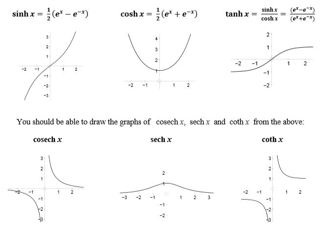
FOR SINH:

The derivative is cosh@ > 0 then the functino is increasing for all @

sinh(0) = 0 so it goes through the origin

sinh@ tends to +/- infinity as x tends to infinity, we have that sinh@ increases steadily to +infinity as @ increases from 0 to +infinity

Also sinh is an odd function, so it mimics itself on rotation by pi around the origin.

FOR COSH:

The derivative is sinh@ > 0 for @ positive.

It is an even function so it is symmetrical about the y-axis, cosh(0)=1.

Whilst cosh@ tends to as @ tends to infinity. Cosh increases steadily from 1 to infinity as @ increases from 0 to infinity.

FOR TANH:

Analysis is similar to those above, we find the derivative 1/cosh^2 > 0 so the function of tanh@ is always increasing.

Tanh is an odd function as tanh(-@) = -tanh(@) this can be shown using the definitions of cosh and sinh. Also tanh(0) = 0 so the sketch goes through the origin.

Behaviour as @ tends to +/- infinity:

Multiplying the top and bottom of tanh by e^-@, as @ goes to infinity then tanh@ goes to 1

Multiplying the top and bottom of tanh by e^@, as @ goes to - infinity then tanh@ goes to -1

Hence deducing that tanh increases steadily from (-1) and (1) passing through the origin as @ increases from (-infinity) to (infinity).

Derivatives of inverse hyperbolic functions:

Derivative of sinh^-1(x): from the sinh graph, for any real value of x there is a unique @ such that sinh@ = x thus arcsinhx = sinh^-1(x) is defined to be the number @ such that

sinh@ = x implies @ = arcsinhx or @ = sinh^-1(x)

Derivative of arcsinh(x) = @, then sinh@ = x and differentiate implicitly, rearrange for d@/dx and use intial defintion to get it in terms of x.

Derivative of cosh^-1(x): when x>1, cosh^-1(x) is defined to be the postive number @ such that

cosh@ = x implies @ = arccosh(x) or @ = cosh^-1(x)

Then for the derivative, cosh@ = x differentiate implicitly, rearrange for d@/dx and use the initial definition to get it in terms of x.

Derivative of tanh^-1(x): the range -1

tanh@ = x implies @ = arctanh(x) or @ = tanh^-1(x)

Then

for the derivative, tanh@ = x differentiate implicitly, rearrange for

d@/dx and use the initial definition to get it in terms of x.

Link between inverse hyperbolic functions and logarithms:

Let x be any real number and @ = arcsinhx then sinh@ = x and cosh@ = (1+x^2)^1/2

then

(e^@-e^-@)/2 = x and (e^@+e^-@)/2 =(1+x^2)^1/2

and adding these two equations gives

e^@ = x + (1+x^2)^1/2 and so taking logarithms gives @ = arcsinh = ln(x + (1+x^2)^1/2)

Proceed similarly for @ = arccoshx to get @ = arccoshx = ln(x+ (x^2-1)^1/2)

Example: Given ln(x^2 +y^2) = 2arctan(y/x), calculate dy/dx and d2y/dx2 in terms of x and y (written up on paper)

Leibniz's Formula:

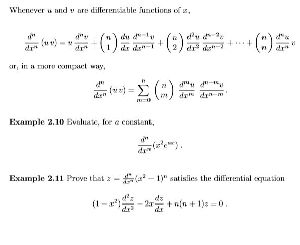
when u and v are functions of x, the nth derivative of the product (uv) can be found by repeated use of the product formula. Alternatively the result can be given by the Leibniz formula.

CHAPTER 3: Integration

When b > a the integral notation is interpreted as the area between y = f(x) and the x-axis and inbetween the lines x = a and x = b. Any of the area lying below the x-axis is counted negatively, that above is counted positively.

If b

CHAPTER 4: First-Order Ordinary Differential Equations

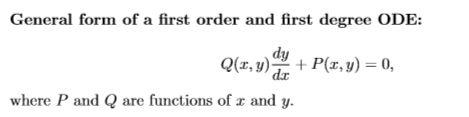
Order and degree of ODE:

The order of an ordinary differential equation (ODE) is the order of the highest derivative that appears in that equation.

The degree of an ordinary differential equation is the power of the highest derivative when the equation has been made rational with respect to the derivatives.

Trivial type:

dy/dx = f(x) where f is a known function involving x alone. Then using the fundamental theorem of calculus, y is the anti-derivative defined to within an arbitrary constant of integration.

A single integration is required to eliminate the anti-derivative dy/dx

The solution involves a single arbitrary constant

Separable equations:

M(x) dx = -N(y)dy

the variables have been separated. You may sometimes be given boundary conditions.

Homogeneous equations:

An equation of the form: dy/dx = f(x,y)

is stb homogenous whenever the function f does not depend on x and y separately but only on their ratio y/x or x/y.

To test if an equation is homogenous, let y =vx, if the resulting expression is of the form f(v) then the eq is homogeneous.

The technique of solution of such equations is to introduce a new dependent variable v, by y=vx so that differentiating wrt x

dy/dx = v + x(dv/dx) by the product rule.

Hence the differential eq dy/dx= f(x,y) = f(v) becomes f(v) = v + x(dv/dx) thus the eq is now separable.

Once separated and solved then substitute back.

METHOD to solve almost homogeneous equations:

These are equations that are similar to dy/dx = (y-x)/(y+x).

The technique is to use a translation and introduce new variables x = X+a and y = Y+b so that the resulting quotient is homogeneous for constants a,b.

Then rewrite the equation and determine the constants a, b so that when solving constants in the numerator and denominator are 0.

Check if it is homogeneous, if so then separate the variables and solve as previously. Don't forget to substitute back for v=y/x

METHOD to solve differential eq using substitution:

For instance when you have dy/dx = ((y-x) + a)/((y-x)+b) where a and b are not the same.

Since we have (y-x) in both the numerator and denominator then we use substitution.

Let z = y-x so differentiating this gives dz/dx = dy/dx -1 and substitute dy/dx = (z+a)/(z+b) into that eq and then simplify.

Once simplified then separate the variables. and solve as previously.

Exact Equations:

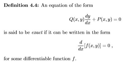
Written up examples for exact equations, need to review these.

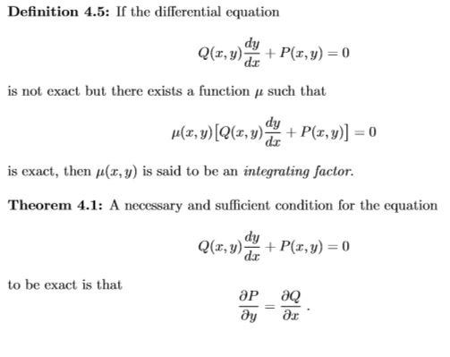
Linear equations:

The differential equations dy/dx + p(x) = g(x) where p and g are given continuous functions of x. Linear of first order.

CHOOSING THE INTEGRATING FACTOR:

The coefficient of dy/dx ought to be 1, if not then divide the entire equation by the coefficient. The integrating factor u(x) = exp(integral(p(t))), where p(t) is the coefficient of y in the initial equation.

The integrating factor is positive and it is determined to within an arbitrary multiplicative constant.

Note: after you have found the integrating factor write that this is to within a multiplicative constant.

METHOD for solving linear equations:

Find the integrating factor, if dy/dx coeff is 1 if not then divide through by the coeff then find IF.

Multiply the entire eq by the integrating factor.

Hence d(u(x)*y)/dx = RHS of the linear eq after multiplied by the IF.

Then integrate.

BERNOULLI'S equation

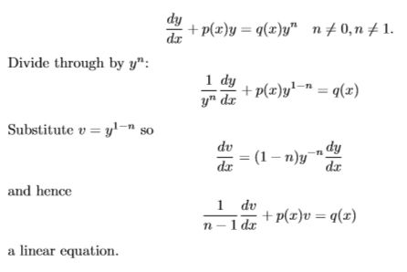
These equations solved by Bernoulli's equation are non-linear but have exact solutions. Follow the above steps once its in the desired form make the coefficient of dv/dx 1 and solve by finding an integrating factor. Once solved for v then substitute back so its in terms of x and y.

KEY POINTS:

Remember to use the correct notation when integrating, this means use a dummy variable t that then changes to x.

Do all the questions on homework sheet again after reviewing these notes above and check them according to the solutions.

Remember after integrating when you write +c state that this is an arbitrary constant.

Remember that after you find u(x), the IF state that this is to within a mulitplicative constant.

Remember to if you introduced new variables write the solution back in terms of x and y.

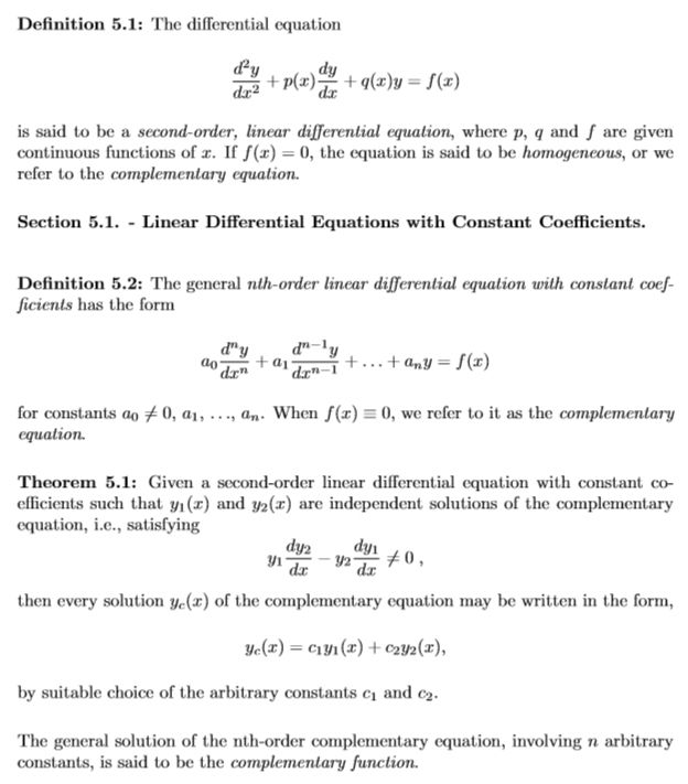
CHAPTER 5: Second Order Differential Equations

Particular integral:

Any solution yp(x) of the nth order linear differential equation with constant coefficients containing no arbitrary constants.

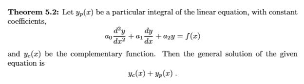
The solution of a general linear differential equation can now be divided into two stages

− finding the complementary function;

− finding a particular integral.

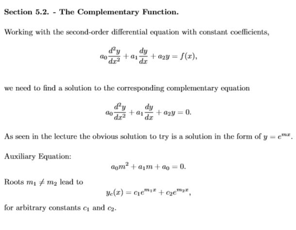
The complementary function:

To find a solution yc(x) which satisfies the given second order DE, so let y = e^mx

Differentiating this gives dy/dx = me^mx and d2y/dx2 = m^2(e^mx).

The substitute all these into the initial eq, since e^mx does NOT equal 0 we get an auxiliary eq that does:

a0m^2 + a1m + a2 = 0

We have a quadratic for m giving roots:

If m roots are real and not repeated then the solutions are y1(x) = e^m1x and y2(x) = e^m2x

Then the CF is yc(x) = c1(e^m1x) + c2(e^m2x) for c1 and c2 arb constants

If m roots are real and repeated then there is only one solution y = e^mx.

Generalising to give y(x) = v(x)e^mx, differentiate this twice, this form must satisfy the DE when substituting back into the intial eq. Some terms cancel giving e^mx(d2v/dx2)=0 so d2v/dx2 = 0 implies v(x) = ax+b for arb consts a,b.

Then the CF yc(x) = c1e^mx +c2xe^mx

If m roots are complex then the solutions are y1(x) = e^m1x and y2(x) = e^m2x where m2 is the complex conjugate of m. Since m1 = a+bi and m2 = a - bi use Eulers Formula: e^i@ = cos@ + isin@

Then the CF is yc(x) = e^a(c1(cos(bx) + isin(bx)) + c2(cos(-bx) + isin(-bx))),

This can be simplified using the fact that cos is even and sine is odd and combining the arbitrary constants.

Reduction of Order Technique:

This is when you have a DE eq where the power is higher than that of 2, we progress similarly. Let y = e^mx and create the auxiliary eq and factorise to find the values of m.

This can also be applied to 2nd order DE with non-constant coefficients.

METHOD for 2nd order DE where the coeffs are non-constants:

These usually ask to show that something is a solution of the following eq, so differentiate it twice, substituting into the initial eq and showing that it satisfies that eq. LHS=RHS.

The seconds part is to determine a second solution:

y(x) = v(x)*x then differentiate this using the product rule

dy/dx = v + x(dv/dx) and d2y/dx2 = 2(dv/dx) +x(d2v/dx2)

So y = vx is a solution provided that is satisfies the eq, substitute into the initial, all v terms cancel.

Let dv/dx = w and assuming x does not equal 0

You get a linear separable eq, gather the terms and integrate.

Remember to substitute back so that the answer is in terms of x.

Particular Integral:

1. If the RHS of a 2nd ODE is an exponential: ce^mx, find the CF, for the PI let yp(x) = Ae^mx for some const A. Then differetiate this twice, yp(x) is a solution of the given eq provided that it satisfies the initial eq. Substitute values in and solve for constant A.

General solution: CF + Ae^mx with the value of A determined

2. If the RHS of a 2nd ODE is a quadratic: ax^2, find the CF, for the PI let yp(x) = ax^2 + bx + c for some consts a,b,c. Differentiate yp(x) and substitute all these into the initial eq, yp(x) is a solution provided that it satisfies that eq. Compare the coefficients to find values for consts a,b,c.

General solution: CF + ax^2 + bx + c with the constant values determined.

3. If the RHS of a 2nd ODE is a trig function: asinbx, find the CF, for the PI

let yp(x) = Acosbx +Bsinbx, differentiate yp(x) and substitute all these into the initial eq, yp(x) is a solution provided that it satisfies the eq. Collect the sin and cos terms and compare the coefficients, thus finding values for A and B.

General solution: CF + Acosbx +Bsinbx with the constant values determined.

How to choose the Particular Integral:

If the particular integral occurs in the RHS of the eq and is a solution of the CF then we introduce a multiplicative factor x.

Also note if the RHS of a 2nd ODE is a hyperbolic function then use the definition to simplify terms.

Examples:

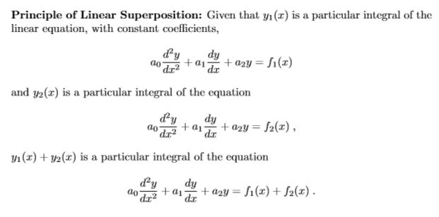
1. When the RHS is the sum of two terms

Find the CF, then consider the PI separately, first the 2nd ODE equal to the first term to find PI and then the 2nd ODE equal to the second term to find PI.

General Solution: CF + PI from first term + PI from second term.

2. When the RHS is the product of two terms: e^ax(cosbx)

Find the CF, for an exponential and trig: combine both and let

yp(x) = e^ax(Acosbx + Bsinbx) differentiate and substitute into initial eq and solve for constants A and B.

General Solution: CF + PI

3. When the RHS is the product of two terms: x^2(e^mx)

Find the CF, for an exponential and quadratic: combine both and let

yp(x) = e^mx(ax^2 + bx +c) differentiate and substitute into initial eq and solve for constants a, b, c

General Solution: CF + PI

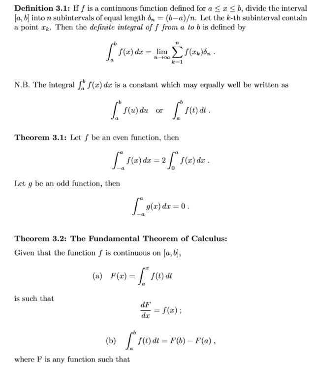
dF/dx = f(x)

For the proof of Theorem 3.1: (interval is in the integral read from bottom to top)

Integral of f(x) in the interval [-a,a] = the integral of f(x) in the interval [0,a] + integral of f(x) in the interval [-a,0]

Then let u = -x so then du = -dx, u is a dummy variable so it does not effect the value of the integral.

Integral of f(x) in the interval [-a,a] = integral of f(x) in the interval [0,a] + integral of f(-u) in the interval [0,a]

So the integral of f(x) in the interval [-a,a] = integral of f(x) +f(-x) in the interval of [0,a]

With f even, f(-x) = f(x),

then integral of f(x) in the interval [-a,a] = two times the integral of f(x) in the interval [0,a]

With f odd, g(-x) = -g(x)

then the integral of g(x) in the interval [-a,a] = integral of g(x) + g(-x) in the interval [-a,a] = 0

If a function is odd no need for integration as this would be 0

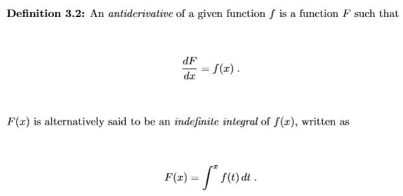
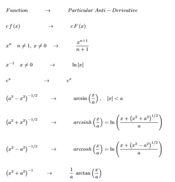
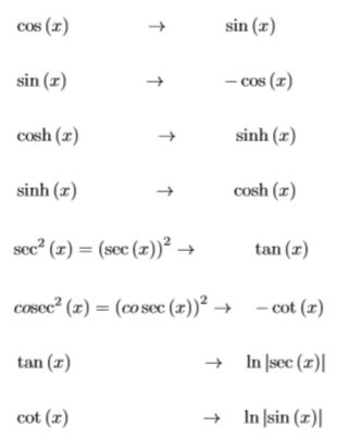
Examples of integrals:

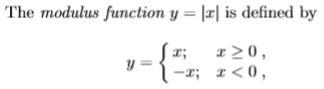
1. Integral involving a modulus function, plotting the graph see where the function crosses the x-axis, so then split the integral into two.

Firstly integrate the function in the mod, from 0 to the point where the function crosses the x-axis

Add this to the integral, from the the point where it crosses the x-axis to the end interval, here you integrate the function reflected in the x-axis. (Negative of the function in the mod).

For instance: integral of |f(x)| in interval [a,b] = integral of f(x) from [a, to point where it crosses x axis] + integral of -f(x) from [the point where it crosses x axis, b]

2. Integral where the function is different for different x values in the domain.

This will give the integral of the first function in the interval of its domain + the integral of the second function in the interval of its domain.

Note if you have a linear expression to the power of n: this will be the reverse of the chain rule.

Method to reverse the chain rule, increase the power of the linear expression in brackets by 1 and multiply by the derivative of the linear function in the brackets and divide by the new power.

Alternatively instead of reversing the chain rule then we can use substitution.

Formally the technique uses a substitution: x = phi(u), so that dx/du = phi'(u).

Then if dF/dx = f(x) , dF/du = dF/dx * dx/du by the chain rule

dF/du = f(x) * dx/du (using the definition)

dF/du = f[phu(u)] * phi'(u)

F(x) = integral of f[phu(u)] * phi'(u) with the limit (phi^-1)x

Examples: different methods for integrating

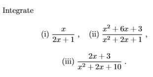
(i) This is an example of rearranging the eq we are given to make it a more familiar one. Now we can use standard forms of integration.

1/2((2x + 1 - 1)/(2x + 1))= 1/2 (1 - (1/(2x+1)))

Now integrate, dont forget +c where c is an arbitrary constant of integration

(ii) Since the numerator has greater terms than the denominator, we can split it into two so that you get 1 + a fraction.

f(x) = 1 + (4x+2)/(x^2+2x+1) now we can factorise to get simpler terms.

f(x) = 1 + (4(x+1)-2)/(x+1)^2 = 1 + 4/(x+1) - 2/(x+1)^2 now when integrating this use dummy variables. When integrated don't forget to include +c where c is an arb const of int.

(iii) For this you can separate the numerator so you get the derivate of f(x) over f(x) this is a known integral form.

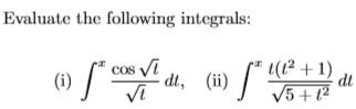
(i) Use substitution: u = (t)^1/2 this can remove the square roots. Find du/dt and substitute into the integral. Now the function is easier to solve.

(ii) The problem in the integral is (5+t^2)^1/2 in the denominator. So use the substitution, let u = in the denominator. Rearrange this to be able to use it in the numerator as well.

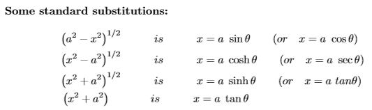
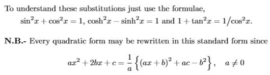
MT171 chapter 1 Introductory CONCEPTS

mt171 Chapter 2 Differentiation

MT171 Chapter 3 Integration

MT171 CHapter 4 First-Order Ordinary Differential Equations

MT171 Chapter 5 second order differential equations