Economics Notes

Seite 1

Economic Issues

Overview

Main points:

- Three central questions economics answers

- What is economics?

- Fundamental concepts if economics

Fundamental Questions:

In the first half of this course, you will learn a model that explains:

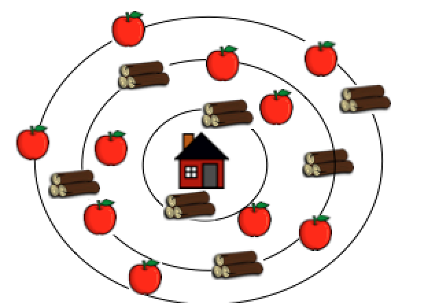
- What gets produced?

- How is it produced?

- Who gets what is produced?

Imagine a Planned Economy

Imagine that there would be a central authority who had to make all these decisions?

This would soon get very messy.

Who makes these decisions in New Zealand?

Theories and Models

In order to answer these big questions we need to simplify. We use theories and models to simplify reality.

Theories are explanations. Models are formal (mathematical) statements of theories, typically about the relationship between two or more variables.

Example of a model: When price goes up - demand goes down.

Demand = A - b*Price

Models

All models simply reality, they are abstractions.

That means all models are wrong, but good models are helpful.

Ceteris Paribus

Ceteris paribus is Latin for all else equal.

Typically outcomes that we are interested in depend on many factors.

When we want to isolate the effect of one single factor we assume that nothing else changes. This is often done implicitly.

Demand = A - b*Price - in this model, we assume that only price changes and that everything else is equal.

Side note: Theory Induced Blindness

Economic analysis focuses on the monetary incentives while all the other factors a held constant (ceteris paribus).

For this reason, economists often forget that other factors matter as well.

Seeing/considering only what your theory focuses on is called theory induced blindness.

Assumptions in Economic Models

We typically assume.

Consumers are rational: they act in a way that best satisfies their wants.

Firms are profit maximising: they act in a way so that they get the highest possible profit.

Competitive markets: many firms, selling identical products to many consumers. All participants have perfect information and firms can freely enter and exit the market.

Is this true? Of course not! But it is very useful.

The Potential of Economics

Economics is a powerful way of thinking about choices.

- Help make better choices

- Help see the world in a new light by giving it structure

What is Economics?

Economics studies how individuals and societies choose to use the scarce resources that nature and previous generations have provided. (Case, Fair, and Oster).

What I think Economics is all about

Economics studies choices under scarcity(1) and how these individual choices lead to higher level (aggregate) outcomes (2).

In the first half of this course we will learn (models of) (1) how consumers and firms make their decisions and

(2) How these individual decisions - through the market and prices - determine

- what gets produced

- how is it produced

- who gets what is produced

Positive and Normative Economics

There are two ways we can study (economic) questions:

Positive economics: Understand and describe behaviour (an economic system) without making judgement.

Normative economics: Evaluate outcomes as good or bad, potentially prescribe courses of action.

In this course we will be focussing on positive economics.

Key Economic Concepts

- Scarcity

- Opportunity Costs

- Diminishing Marginal Returns

Scarcity

Scarce: Limited. Scarcity: Wants > resources

The basic economic problem, the gap between scarce resources and theoretically limitless wants.

Requires people to make decisions about how to allocate resources efficiently, in order to satisfy basic needs and as many additional wants as possible.

Economists study situations in which we can't satisfy all our wants. Therefore we have to make trade-offs.

Opportunity Costs (1)

Opportunity costs: The cost of the best alternative that we have to give up when we make a decision.

Paul's opportunity costs for going to college include not only the tuition fee but also the money he could have earned if he would have worked.

Imagine Paul wouldn't be able to find a job. How could this influence his opportunity costs of going to college?

Economists argue that you should consider opportunity costs and assume in their models that people do.

What are the opportunity costs of going to the lecture?

Are the opportunity costs higher when the lecture is at 7am?

Marginalism (1)

Marginalism is the process of analysing the additional or incremental costs or benefits arising from a choice or decision.

Marginalism (2)

Economists argue that you should consider the marginal (as opposed to the average) costs and benefits of their decisions.

Imagine you are about to but an ice cream for $3 and the seller offers you a special deal of two ice creams for $4 dollars.

Marginal cost: $3 $1

Marginal benefit: ? ?

Choices

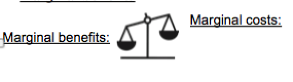
Rational consumers and profit maximising firms makes choices by weighing marginal costs against marginal benefits.

This way of thinking is not limited to monetary costs and benefits.

Should Paul go to College?

Marginal Benefits Marginal Costs

Higher salary Forgone salary

Learn new things Studying is exhausting

Getting student discounts Cost of school books

Aggregate Outcomes

Paul's behaviour also depends on what other actors (e.g. potential students, employers) are doing?

Paul's decision what to study also depends on how much he can earn in a particular profession.

How much a profession pays depends - among other things - on how many other people want to work in this profession.

Wages get determined on the labour market.

Markets

A market is a situation or institution through which a voluntary exchange takes place.

In the labour market, you exchange labour for a wage.

A market need not be a physical location

e.g. A fruit market, the NZSX, TradeMe

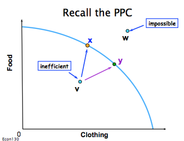
The Production Possibility Curve (PPC)

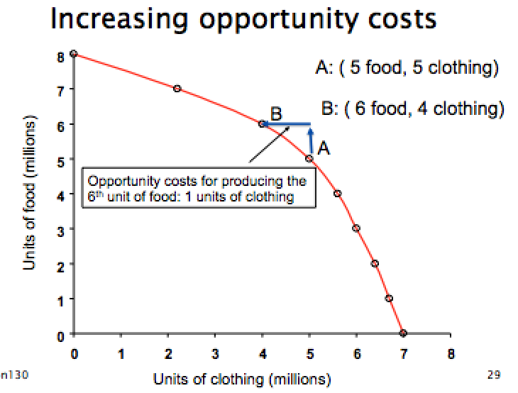
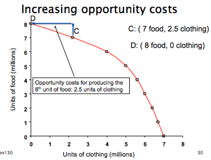
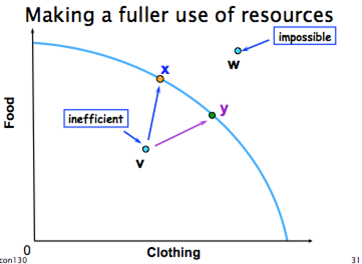
The production possibility curve shows the maximal mix of outputs that an economy can achieve.

The PPC demonstrates the concepts of:

- Scarcity

- Trade-offs

- Opportunity costs

We have a simple 2 good economy

- The goods are food and clothing

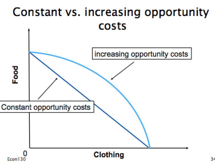
Laws of increasing opportunity costs - producing more will cost more than average.

As production increases, the opportunity cost does as well.

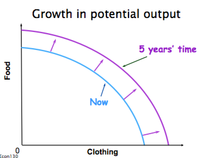
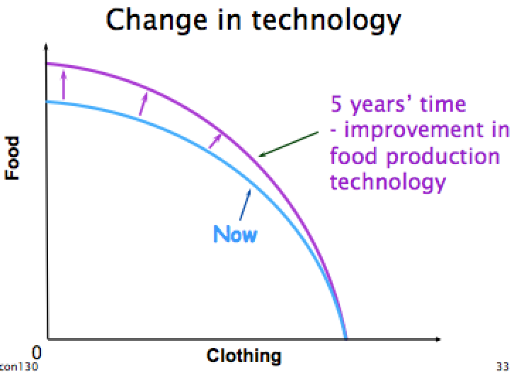
Economic

growth

-What does it mean?

-Who benefits? Everyone?

-Who loses?

-Who and how are these decisions

made/arbitrated (in local, block or global economies/polities)?

Seite 2

Consumer Choice

Overview

Main Points

- The budget set and budget constraint

- The preferences and utility

- The optimal consumption plan

- Income and substitution effect

- Choice between leisure and consumption

- Choice between consumption today and consumption tomorrow

What to consume depends on:

-What the consumer can afford (budget)

- The consumer's preference (taste)

What can the consumer afford?

In this model, we will only consider income and not wealth.

We will also assume that the consumer spends all their income on only two goods.

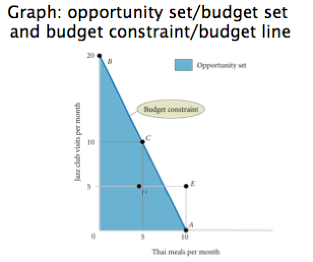
Example: Meals and Jazz

Income (I): $200

Good X: Thai meals ($20 per meal)

Good Y: Jazz visit ($10 per ticket)

Assuming all income is spent, these are the possibilities:

$200 = $20*Meals + $10*Jazz

General Version:

The Budget Set/The Opportunity Set

Income and prices together determine the possible consumption bundles - combinations of goods - that a consumer can afford.

The budget set consists of all the different bundles of goods a consumer can afford.

It can be shown graphically as an area e.g. the triangle.

The Budget Constraint/Budget Line

The budget constraint (BC) shows the different bundles a person could buy when they spend all their income.

It separates the affordable bundles from the unaffordable bundles.

It represents the limit or constraint a consumer has on their spending.

Note that it is also sometimes called a budget line.

Changes in Income

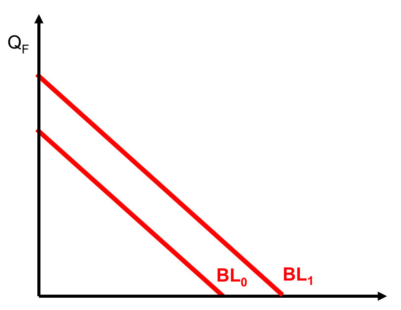
Changes in income shift the budget line parallel to the original, because the slope is unchanged. An increase:

- expands the consumers' opportunity set

- means they can buy more goods

- makes consumers better off

If income decreases, the BL shifts in toward the origin, parallel to the old BL.

Changes in Price of a Good

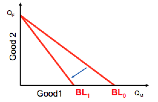
An increase in the price of one good rotates the budget line. The figure below shows how the budget line changes if the price of Good 1 increases (p1>p0)

Relative Price

A relative price is the price of one good in terms of another good.

Example:

The relative price of one thai meal ($20) is two jazz club visits ($10), because you would have to give up two jazz club visits for each meal ($20/$10 = 2)

The relative price of one jazz club visit is half a meal, because you would have to give up half a meal for one jazz club visit ($10/$20 = 0.5)

Relative prices determine the slope of the budget constraint.

What are the Consumer's Preferences?

Again. we are in a model where there are only two goods.

We don't explain where preferences come from, but discuss a way to represent them.

Utility

Utility is a concept that measures how much satisfaction/benefit an alternative yields.

Economists express consumers' preferences with the concept of utility.

Example:

If Paul prefers one apple over one pear, we sat Paul get's more utility from an apple than from a pear.

If Paul gets twice as much satisfaction from an apple than from a pear, we can say that: Uapple = 2*Upear

For example: Uapple = 10 Upear= 5 or Uapple = 20 Upear = 10

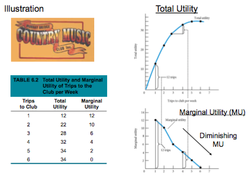
Total and Marginal Utility

The satisfaction obtained from all goods is called total utility.

We refer to the satisfaction derived by an additional unit of a good as marginal utility.

The law of diminishing utility states that in general, the marginal utility of a good decreases as the consumer buys more of a good (or service).

Indifference Curve

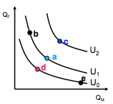
An indifference curve is a graphical representation of bundles that give a consumer the same level of utility.

Features of an IC:

- An IC shows a particular level of utility

- Higher indifference curves represent greater utility

- Their slope gets flatter to the right (Due to DMU)

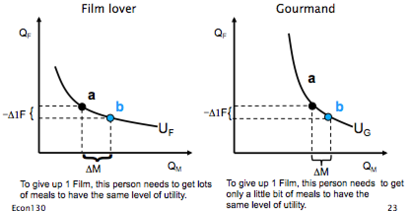
- The shape of the indifference curve reflects the person's preferences

Indifference Curves

Different preferences appear as different shaped ICs

Marginal Rate of Substitution

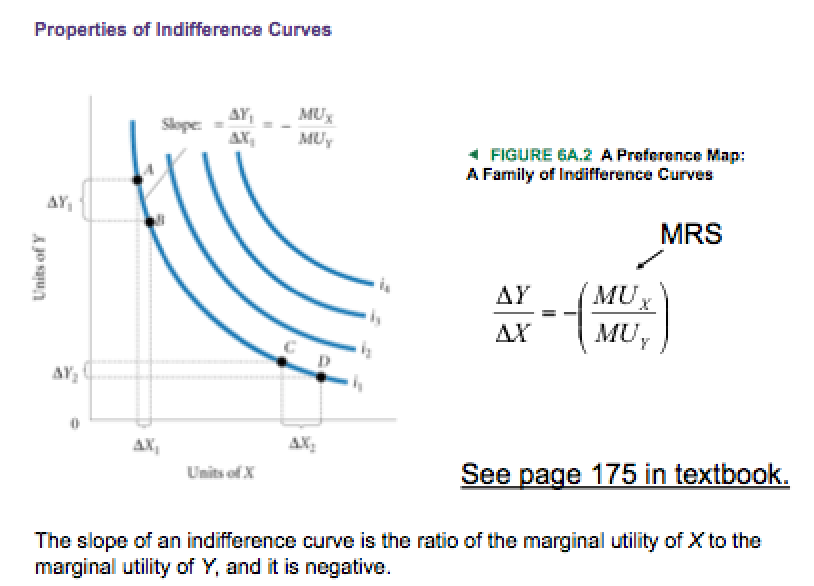
The marginal rate of substitution (MRS) is the rate at which a consumer is ready to give up one good (Y) in exchange for another good (X) while maintaining the same level utility. Thus, the MRS is defined as MU(x)/MU(y)

When MU(x)/MU(y) = 4, for example, the household would be willing to trade 4 units of Y for 1 unit of X. Such a trade would leave the household with the same level of utility.

The negative of the MRS is the slope of the indifference curve.

We will now look at... How to choose optimally?

Here we will look at limited budgets and preferences at the same time.

We first look at an example to understand the intuition.

Then we look more formally on how to model optimal choice.

Optimal Choice

We ask the question: given a limited budget, which bundle of goods does the consumer purchase to maximise his or her total utility.

Consider Frank, who has budget of $21 and wants to spend it on going to the club (good 1) and seeing basketball games (good 2).

How to allocate income to maximise utility?

We want to get the highest possible marginal utility per dollar!

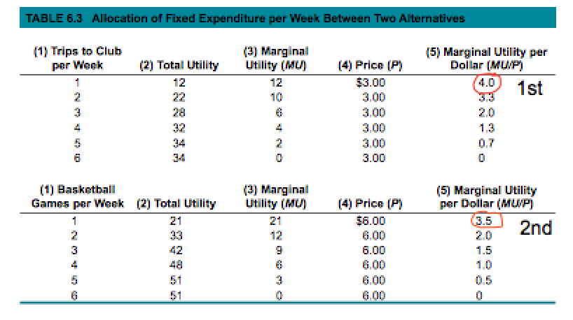
The Equi-Marginal Principle (1)

A consumer maximises his utility where he receives the same marginal utility per dollar from both goods:

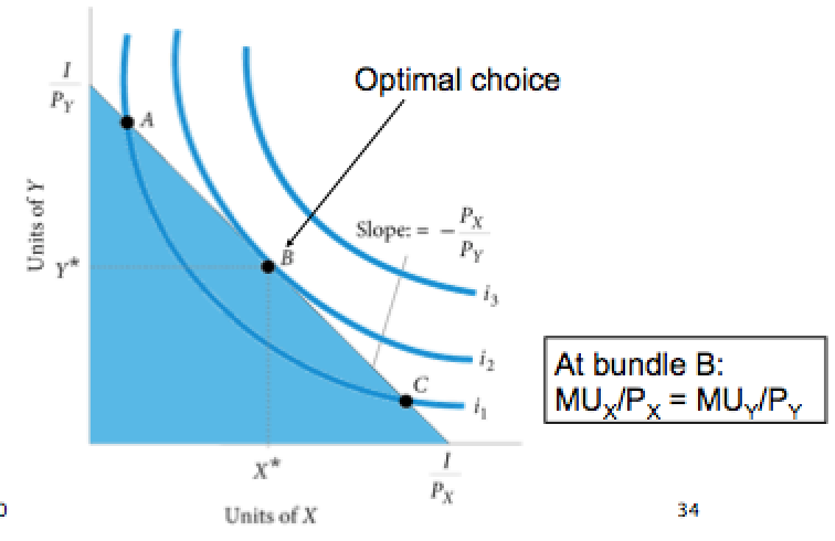
MU(x)/P(x)=MU(y)/P(y)

If the consumer receives more utility per dollar from consuming good X than good Y, then he can increase his utility by buying more X and less Y.

- If he buys more X, MU(x) falls due to diminishing marginal utility

- If he buys less Y, MU(y) increases

- The consumer should continue to change their spending pattern as long as MU(x)/P(x)>MU(y)/P(y)

The Equi-Marginal Principle (2)

The consumer should continue to adjust his consumption so that MU(x)/P(x) falls and MU(y)/P(y) rises until they are equal.

This is called the equi-marginal principle.

A bundle where MU(x)/P(x) = MU(y)/P(y) means that person derives that same satisfaction per dollar of expenditure from each good.

With such a bundle, there is no reallocation that can increase their utility (assuming that they are spending all their income already).

Optimal Choice in a Graph

Optimal choice is at the point where our budget line is tangent to the highest possible indifference curve.

Substitutes and Complements

Substitutes - goods that can serve as replacement of one another; when price of one increases, demand for the other increases.

Example: German and Japanese cars.

Complements - goods that "go together", an increase in the price of on results in a decrease in the price of the other (and vice versa)

Example: X-box, xbox games

Normal Goods

A normal good is a good for which demand goes up when income is higher and for which demand goes down when income is lower.

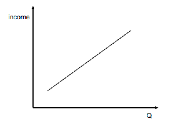
Normal Goods in the Budget Constraint Framework

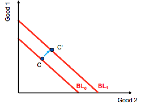
When both goods are normal, an increase in income induces a new choice. At this optimal new choice, the quantity demanded for each good increases.

Inferior Goods

An inferior good is a good for which demand falls when income is higher and for which demand rises when income is lower.

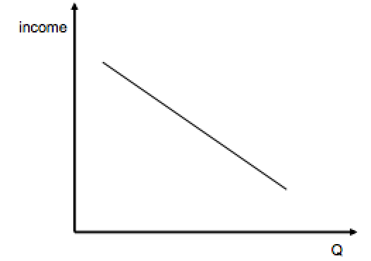
Inferior Goods in the Budget Constraint Framework

When good 1 is a normal good and good 2 is an inferior good. After a raise in income, at the new optimal choice point D, less of good 2 is demanded.

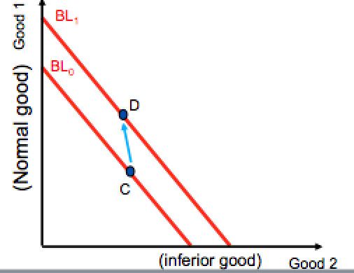
Whether a good is a normal or inferior good depends on the specific circumstances and can change with income.

Normal good: demand goes up when income goes up

(Laptop)

Inferior good: demand goes down when income goes up

(Bus ticket)

Real Income

Real income is the set of goods and services available to a household as determined by prices and money income.

Or, real income is income expressed in things you can buy.

In meals ($20)/jazz club ($10) example where the money income is $200, the real income is 10 meals or 20 jazz club tickets.

Real income: Monetary income/price level

Adjustment to a Price Change

A change in price of one good has two effects.

1) It changes the relative prices.

The good is now cheaper relative to the other good.

The reaction to this is called the substitution effect.

2) It changes the real income.

When a good gets cheaper you can buy more products overall.

When a good gets more expensive you can buy less overall.

The reaction to this is called income effect.

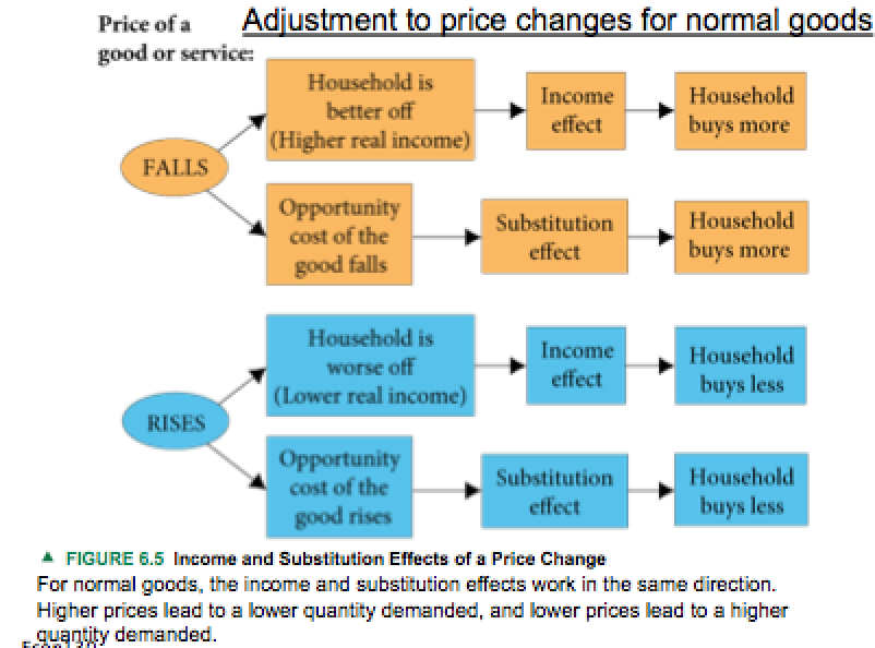
Adjustment to a Price Change for an Inferior Good

Price of inferior good decreases:

Substitution effect: Good gets cheaper relative to other goods (opportunity costs fall)

- Household buys more

Income effect: Household's real income increases

- Household buys less of it

Price of inferior goods increases:

Substitution effect: Good gets more expensive relative to other goods (opportunity costs fall)

- Household buys more

Income effect: Household's real income increases

- Household buys less of it

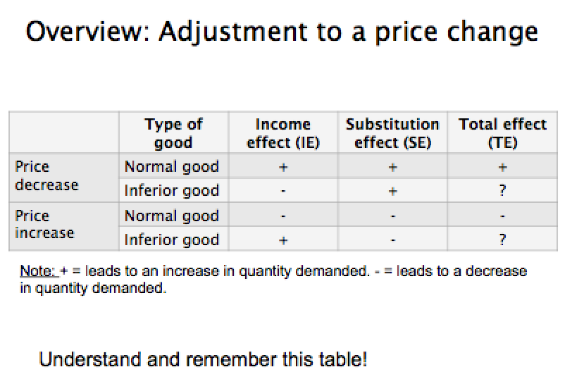
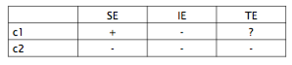
How to Remember SE and IE

Substitutions effect is intuitive:

As price goes up - less demand (SE is negative)

As price goes down - more demand (SE is positive)

Income effect is intuitive for normal goods:

As price goes up - less demand (IE is negative)

As price goes down - more demand (IE is positive)

Income effect is not intuitive for inferior goods

As price goes up - more demand (IE is positive)

As price goes demand - less demand (IE is negative)

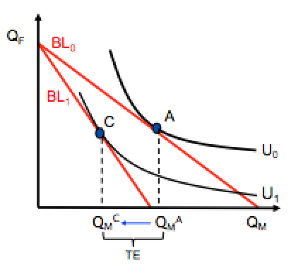
Total Effect (Normal Good)

Say Pm↑ increases.

This leads to a new Budget Line (BL1) and the optimal consumption changes from A to C.

The total effect in quantity consumed of product M is the deduction QmA to QmC.

We will now decompose the total effect into the substitution effect and income effect.

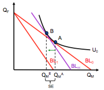
Substitution Effect (Normal Good)

What would be the consumption with the new relative prices (slope of BL1) and the old utility level (U0)?

Approach: Shift a hypothetical budget line (BLH) parallel to the new budget line (BL1) until it is tangent to the old indifference curve (U0).

The change in quantity between bundle A and B (BLH is tangent to U0) is the substitution effect.

The SE is for both normal inferior goods negative for a change in its own price.

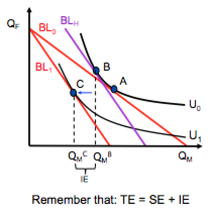
Income Effect (Normal Good)

The IE reflects the change in quantity demanded due to the fall in real income at constant relative prices. It is as if the only thing that has changed is income.

The IE is the change in quantity demanded of good M after we have accounted for the substitution effect.

It is the move from QmB to QmC.

Because M is a normal good, the IE is negative. That means a reduction in real income leads to reduction in demand.

Remember that: TE = SE + IE

The Labour vs Leisure Tradeoff

We will now apply this utility maximisation framework to model people's choice between work and leisure.

We will again assume that people don't save.

The Labour and Leisure Choice (1)

Why work? Our model assumes people work to earn income which they use to buy products.

Workers are interested in the real wage.

The real wage is the nominal wage adjusted for inflation.

W = nominal wage (after taxes)

P = price of consumption

Real wage = w = W/P

An hour of work buys $w (W/P) units of goods.

The Labour and Leisure Choice (2)

People face a tradeoff in the choice of consumption goods (leisure or goods purchased from labour income).

The set of choices is limited by the amount of time a person has available to them - 24 hrs in a day.

So the wage implicitly gives the opportunity cost of leisure in dollar terms: an hour of leisure means an hour less work - you give up $w.

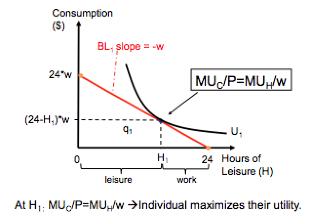
The Ideal Mix of Labour and Leisure (1)

You can think of the tradeoff as a tradeoff between leisure (H) and consumption that is made possible through paid work.

The best choice equates the benefit from an extra hour of work (in additional consumption) with the marginal cost of that hour (the value of an extra hour of leisure).

MU(c)/P=MU(h)/w - real wage

This is another application of the equi-marginal principle.

The Ideal Mix of Labour and Leisure (2)

Labour Force Particpation (1)

We can extend the labour leisure model to explicitly incorporate other factors that can influence one's decision to work.

We will now look how extra costs of working (e.g. the cost of commuting) and an non-labour income would affect the decision to work.

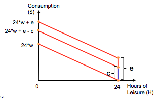
We do this incorporating the cost of working (c) and non-labour income (e) in the budget constraint.

Labour Force Participation (2)

- Non-labour income (e)

- Costs of taking a job (c) - assume these are fixed costs.

Response to a Wage Rise

A higher wage rate (W↑):

1. Increases the relative return to working. It is a price effect that encourages people to work more (take less leisure, H↓). This is the substitution effect.

2. Increases people's real income. Assuming leisure is a normal good (and work is an inferior good), income increases allows people work less (choose more leisure), H↑. This is the income effect.

- The total effect of a wage rise on hours worked is not straight forward.

Response to Wage Fall

A lower wage decreases the relative return to working.

- reduction of working hours (Substitution effect)

A lower wage also decreases real income.

- increase in of working hours (Income effect)

The total effect on working hours can be positive or negative.

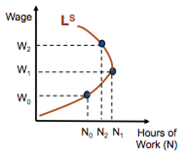
Backward-bending Labour Supply Curve

When leisure is plentiful, and other goods are scarce, people place a low value on leisure and a high value on work (i.e. other goods).

Initially, increasing the wage has a strong opportunity cost effect. With a lot of leisure already, the worker values the additional goods more than the leisure.

At higher wages, leisure becomes more scarce.

Ultimately, a W↑ results in fewer hours of work being supplied: the L(s) curve is backward-bending.

The individual prefers to use the extra purchasing power of the wage rise to 'buy' leisure rather than other goods.

The Consumption-Saving Choice

Another application of the constrained choice framework to individual decision making problems is the savings decision.

We will model the saving decision as choice between two goods: goods today and goods in the future.

Saving

The savings decision is a choice between two goods: goods today and goods in the future.

Three determinants of saving are:

1) income (from which people save)

2) the interest rate (which yields a return to saving)

3) how much people care about current consumption relative to future consumption (time preference).

The Saving Decision

Suppose a person has a working period and a retirement period. They earn income of w(t) in the period t, and that the real interest rate is r.

If they do not save in period 1 they have only w(2) to consume in period 2 (their retirement).

If the person save all they earn (w1) in period 1 (their working age) they can consume (w1(1+r)+w2 in period 2.

Together lifetime income and the real interest rate define a (simple) lifetime budget constraint.

The Inter-Temporal Budget Constraint

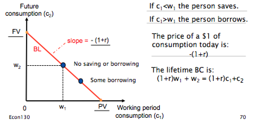
The inter-temporal (or lifetime) budget constraint constraint (BC) represents the possible combinations of consumption in the working period and in the retirement period.

- If a person consumes all their income during the working period there are no saved funds available for retirement.

The BC shows a trade-off: a person can consume less now and more later, but they must wait to consume.

The relative cost of consuming $1 in period 1 is $(1 + r) lower consumption in period 2.

The Saving Decision (1)

The person earn w(1) in period 1; they can consume it (c1) or save it (for c2). They can also borrow against w2.

The Decision - for a Saver

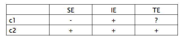
What happens if I increases (i↑) Assume that c1 and c2 are normal goods.

For a saver: i↑ - real income ↑

The Decision - for a Borrower

What happens if I increase (i↑)? Assume that c1 and c2 are normal goods.

For a saver: i↑ - real income ↓

Seite 3

Producer Choice

Overview

Main Points:

- The production process (costs)

- Short run decisions (quantity)

- Long run decisions (quantity)

What is a Firm's Objective?

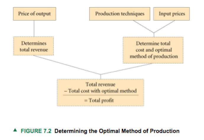
We begin with the assumption that a firm aims to maximise profits.

What is profit, and how do firms maximise it?

Revenues

- the amount a firm earns. TR = P x Q

Costs

- the costs of production. TC = VC + FC = MC x Q + FC

Profits

- the difference between revenue and costs P = TR - TC

(Losses are negative profits, where costs exceed revenues)

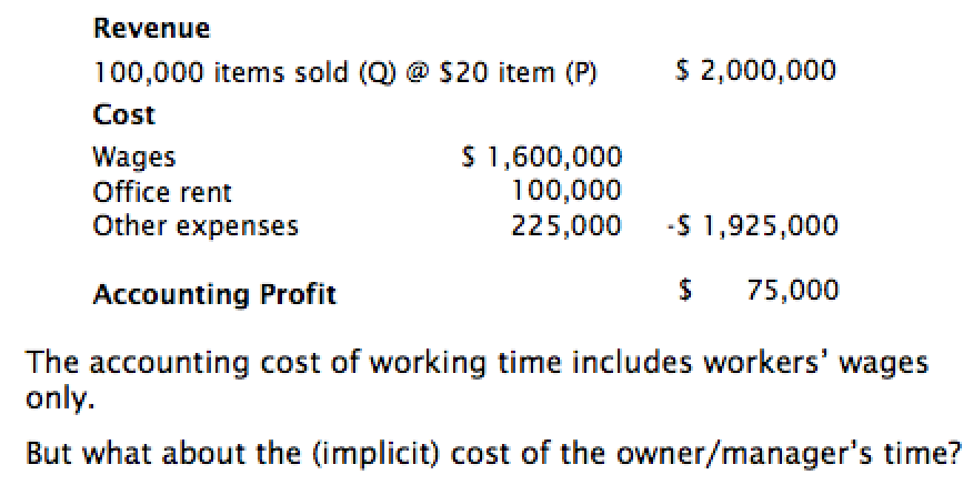
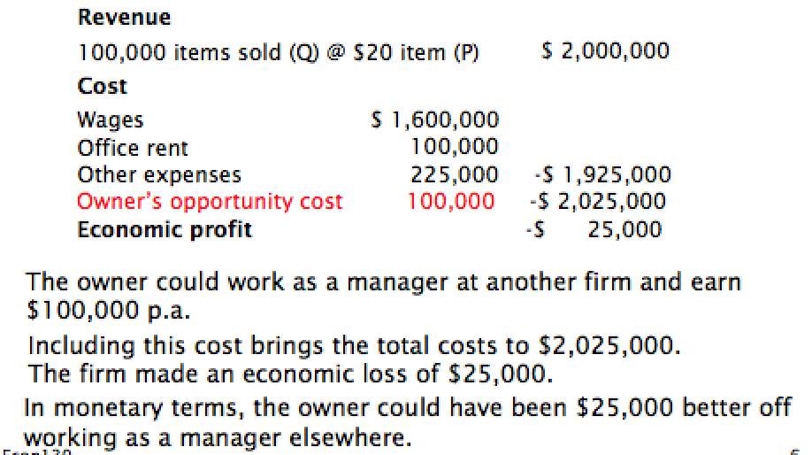
Economic vs. Accounting Profit

Economic profit = total revenue - total economic costs

Accounting profit = total revenue - total accounting costs

Accounting costs: out-of-pockets costs

Economic costs: Accounting costs + opportunity costs of all factors of production

If not mentioned otherwise, costs refer to economic costs.

Example: Accounting Profit

Example: Economic Profit

The Short Run and the Long Run

The short run is a time period during which some inputs are fixed.

- Those factors fixed in the short run generate short-run fixed costs

- Labour and raw materials are the principal variable inputs

- Capital is typically regarded as a fixed input

The long run is a time period during which no inputs are fixed; all inputs can be changed.

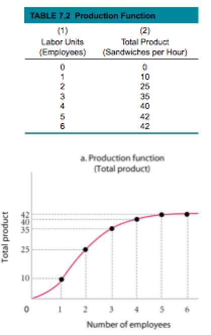
Production Function

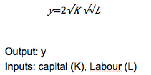
A production function is a numerical or mathematical expression of a relationship between inputs and outputs.

Example:

We start with the sandwich shop example.

Firm with one variable factor of production in the short run.

Variable factor of production: labour

Fixed factor of production: table, grill, etc.

Marginal Product and Average Product

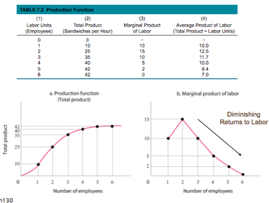
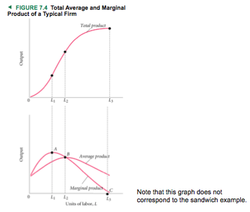
Marginal Product - the additional output that can be produced by adding on more unit of a specific input, ceteris paribus.

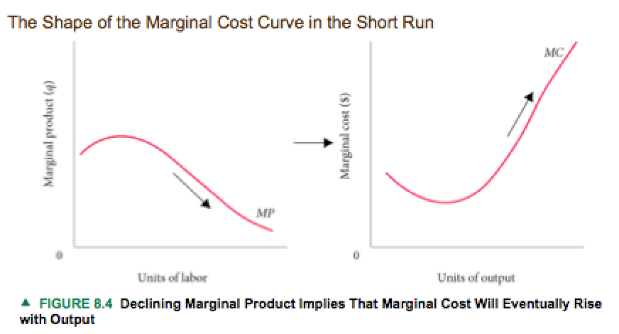
Law of Diminishing Returns - when additional units of a variable input are added to fixed inputs, after a certain point, the marginal product of the variable input declines.

Average product - the average amount produced by each unit of a variable factor of production

Average product of labour = total product/total units of labour

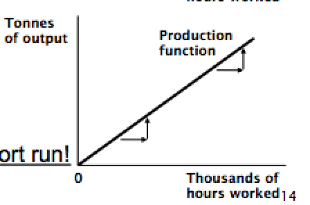
Other Shaped Production Functions

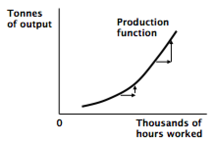
Increasing Marginal Product

- doubling an input more than doubles output

Constant Marginal Product

- doubling an input doubles output

Two Variable Factors of Production

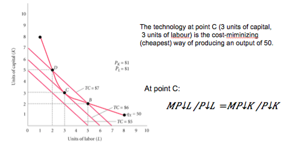
What is the combination of inputs that produces the desired level of output at the lowest cost?

The optimal combination of factors of production depends on their (joint) productivity and the factor costs.

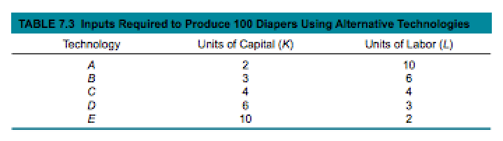
Example Diaper Manufacturer

Two variable inputs: capital (K) and labour (L)

Possible combinations to produce 100 diapers:

Iso = equal

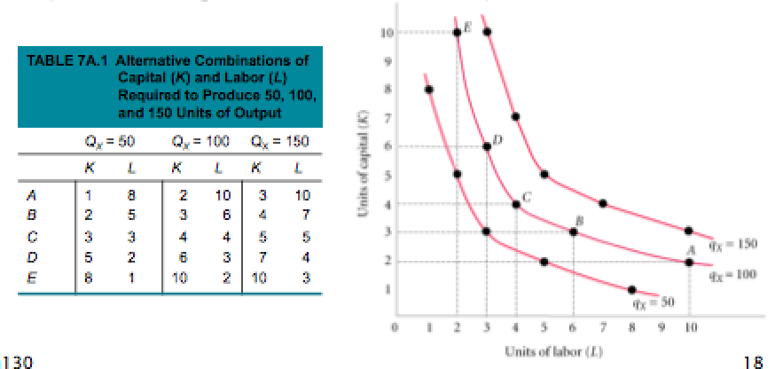
Production Isoquant

An isoquant is a graph that shows all the combinations of capital and labour that can be used to produce a given amount of output.

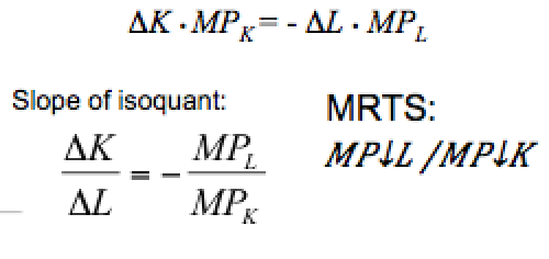
Marginal Rate of Technical Substitution

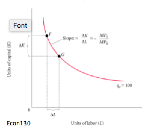
Marginal rate of technical substitution (MRTS) is the rate at which a firm can substitute capital for labour and hold output constant.

For output to remain constant, the loss of output from using less capital must be matched by the added output produced by using more labour.

Isocost Line

An isocost line is a graph that shows all the combinations of input Y (capital) and input X (labour) available for a given total cost.

(P(k) · K)

+ (P(l) ·

L)

= TC

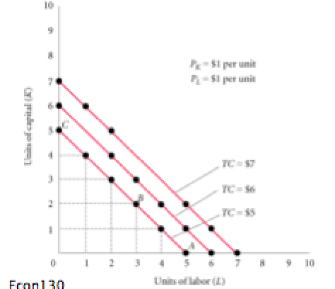
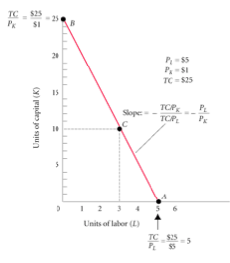
Isocost Line and Changes in Price

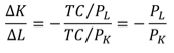
Slope of Isocost Line:

Cost-Minimisation with Two Variable Inputs

The cost-minimising combination of inputs is at the point where

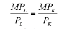
This is an application of the equi-marginal principle.

That is, the marginal product per dollar should be equalised across all (variable) inputs.

Otherwise the firm could spend more on the input with the high marginal product per dollar and less on the input with the low value, and increase output.

Finding the Least-Cost Technology with Isoquants and Isocosts

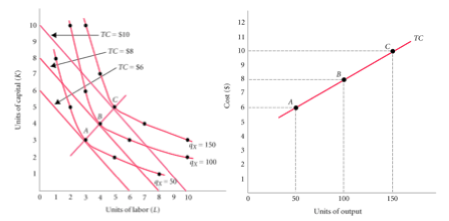
Derriving the Production Function

The production function shows the relationship between output and cost given the cost minimising combination of capital and labour at each output level.

Short Run Decisions

Recall:

- The firm wants to maximise profits

- In the short run, firms face fixed costs and variable costs

- If the firm needs two (or more) factors of production, the variable costs reflect the cost minimising way to produce a given quantity.

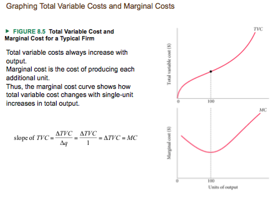
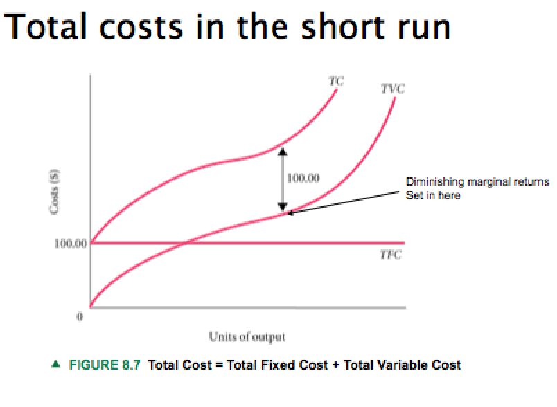
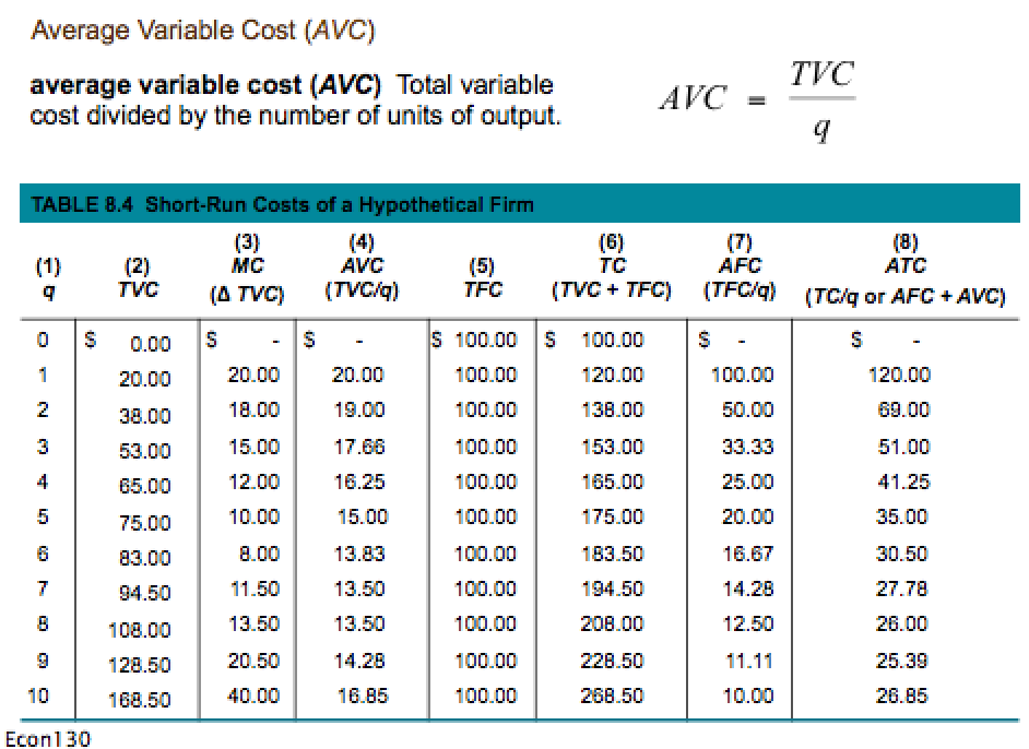
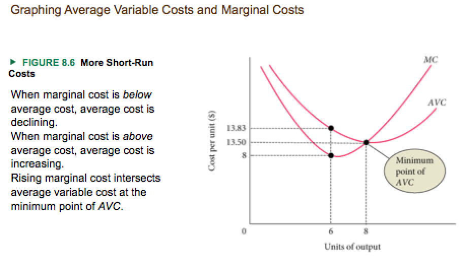
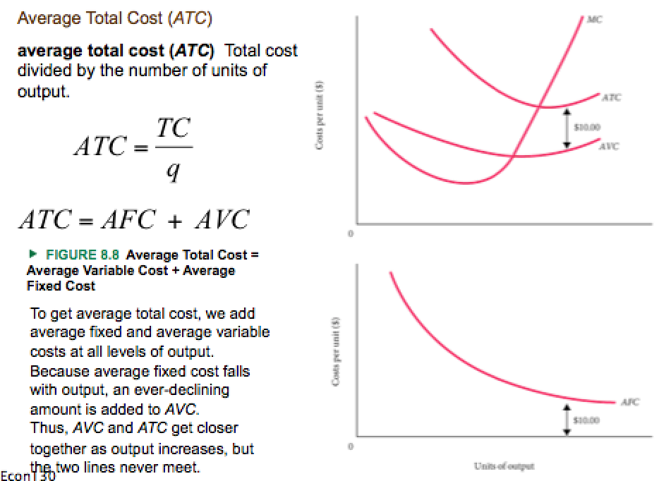
Costs in the Short Run

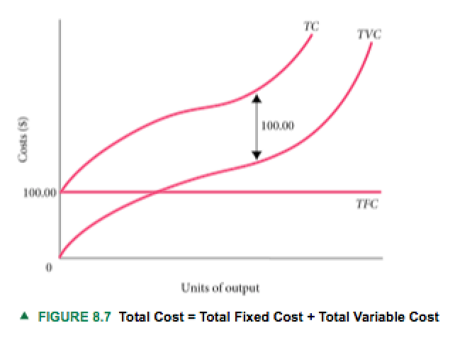
Fixed costs are any cost that does not depend on the firms' level of output. These costs are incurred even if the firm is producing nothing.

Variable costs depend on the level of production chosen.

Total costs are total fixed costs plus total variable costs.

TC = TFC + TVC

Total Costs in the Short Run

How Much Should the Firm Produce?

Recall that the firm wants to maximise profits.

At which quantity produced (level of q) does the firm maximise profits?

Recall that profits are: P = TR - TC

Where TR = P x Q and TC = VC + FC = MC x Q + FC

So we need to know the price P to find the Q that maximises profits.

Perfect Competition

We assume that firms are in perfect competition. That means that there are many firms that produce identical products and firms can freely enter and exit the market.

Perfect competition implies that firms are price takers, i.e. they can sell their products at the market price only ( - if they would ask 1 cent more, everyone would buy the product somewhere else).

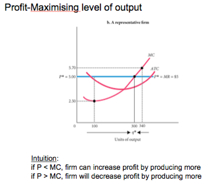
Profit-Maximising Level of Output

The profit-maximising output level for all firms is the output level where MR = MC.

In perfect competition, MR = P. Hence, for perfectly competitive firms, we can rewrite our profit-maximising condition as P = MC.

Long Run Costs and Output Decisions

Recall that in the long run

- all costs are variable (there are no fixed costs)

- firms can freely enter and exit the market

We start off by looking at the firms decision in the short urn and their implications for the long run.

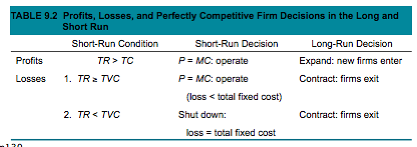
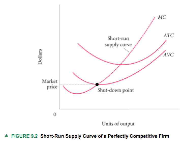
Firms Decision in the Short Run

If P>ATC, produce until P = MC - make a profit

If P<ATC and P>AVC, produce until P = MC

- make a loss <fixed costs

If P<AVC, stop production

- make a loss = fixed costs

Long Run Costs

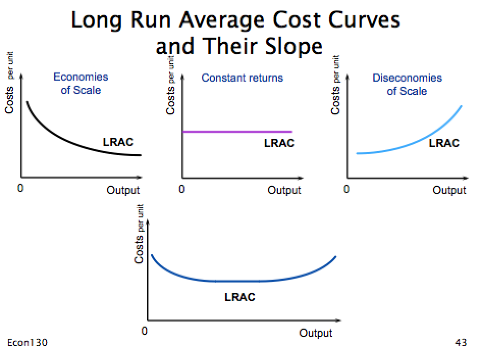
Increasing Returns to Scale, or economies of scale:

- An increase in a firm's scale of production leads to lower costs per unit produced.

Constant Returns to Scale:

- An increase in a firm's scale of production has no effect on costs per unit produced.

Decreasing Returns to Scale, or diseconomies of scale:

- An increase in a firm's scale of production leads to higher costs per unit produced.

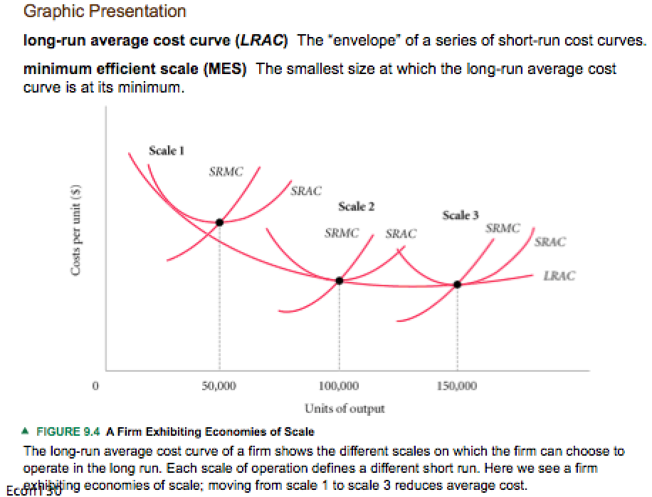
Long-Run Average Cost Curve

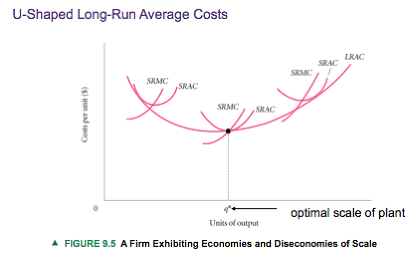
A firm's long-run average cost curve (LARC) tells us the average cost of producing an associated level of output (in the long run, when all costs are variable).

The optimal scale of the plant is the scale of the plant that minimises the long-run average costs. It is the minimum of the LARC.

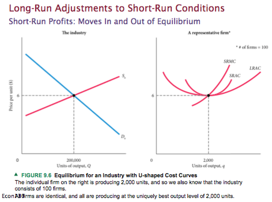
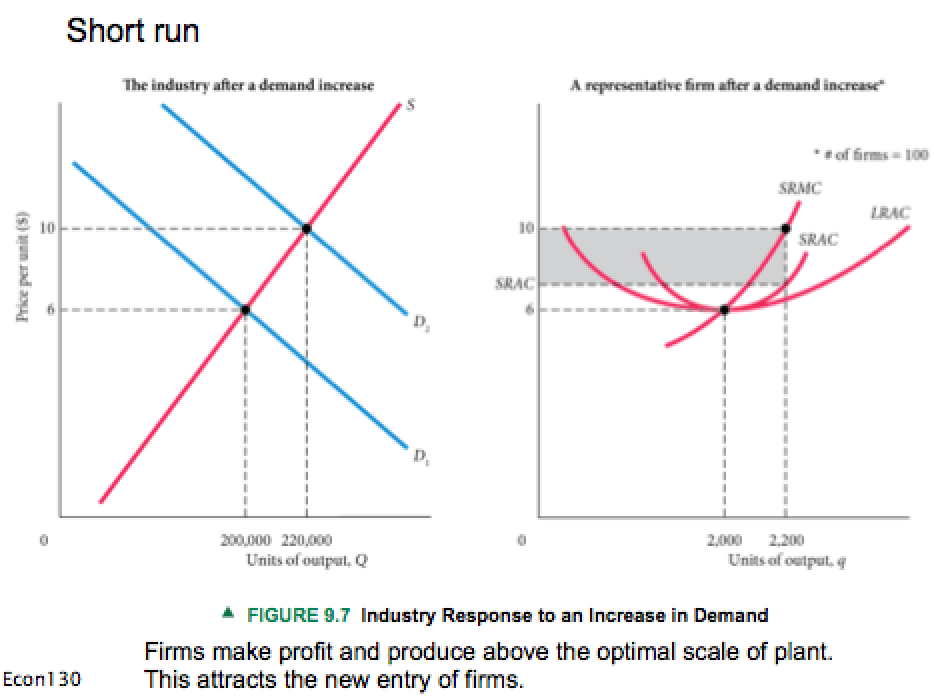
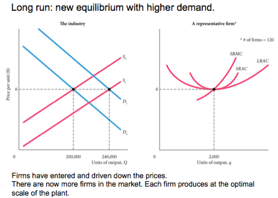
In equilibrium, each firm has:

SRMC = SRAC = LRAC

Firms make no excess profits so that:

P = SRMC = SRAC = LRAC

and there are enough firms so that supply equals demand.

What does the Firm Choose?

One variable factor of production (input):

Firm chooses the quantity produced (Q) that maximises profit.

Two variable factors of production (typically capital and labour):

Firm simultaneously chooses quantity produced (Q) and combination of factors of production that maximise profit.

Seite 4

Equilibrium

Main points

- demand and supply

- equilibrium and adjustment

- the price mechanism

Some Key Terms

Market

- a process for voluntarily exchanging goods or services where prices adjust to reconcile competing demands.

Demand

- the quantity that buyers wish to purchase at each conceivable price

Supply

- the quantity that sellers wish to sell at each conceivable price

Equilibrium Price

- price at which quantity supplied = quantity demanded

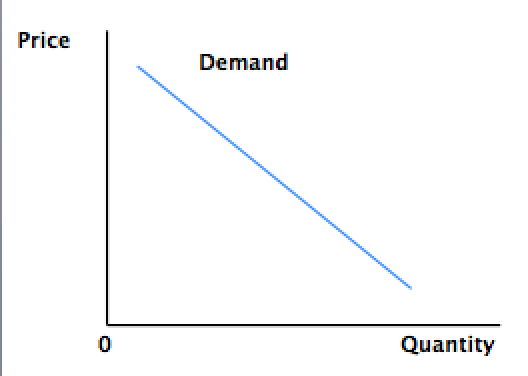
The Demand Curve

The demand curve shows the relation between price and quantity demanded holding other things constant.

"Other things" include:

- consumer preferences

- consumer incomes/credit

- the price of related goods

- demographics

- expectations

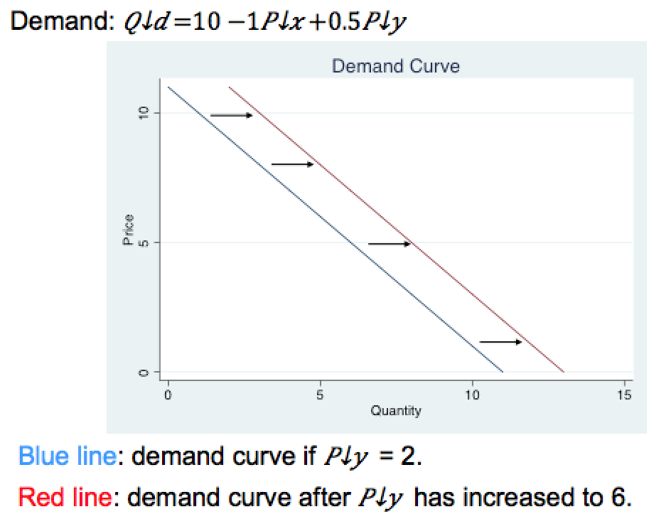
Changes in these other things affect the position of the demand curve.

The Demand Curve - Math

The demand curve can be expressed as a mathematical function.

For example:

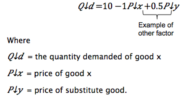
Changes in other factors lead to a shift of the demand curve.

The Supply Curve

The supply curve shows the relation between price and quantity supplied holding other things constant.

"Other things" include:

- input costs

- technology

- government regulations

- alternative production opportunities

- aims/objectives

- expectations

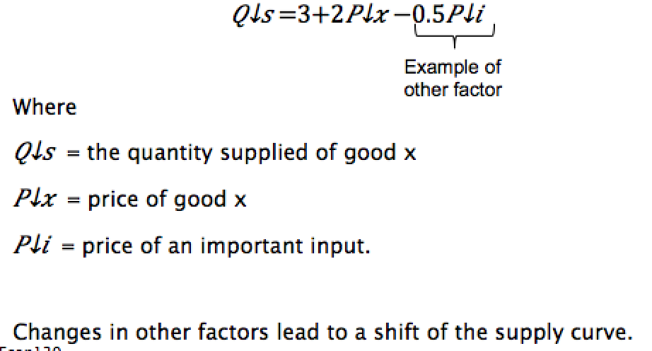
Changes in these other things affect the position of the supply curve.

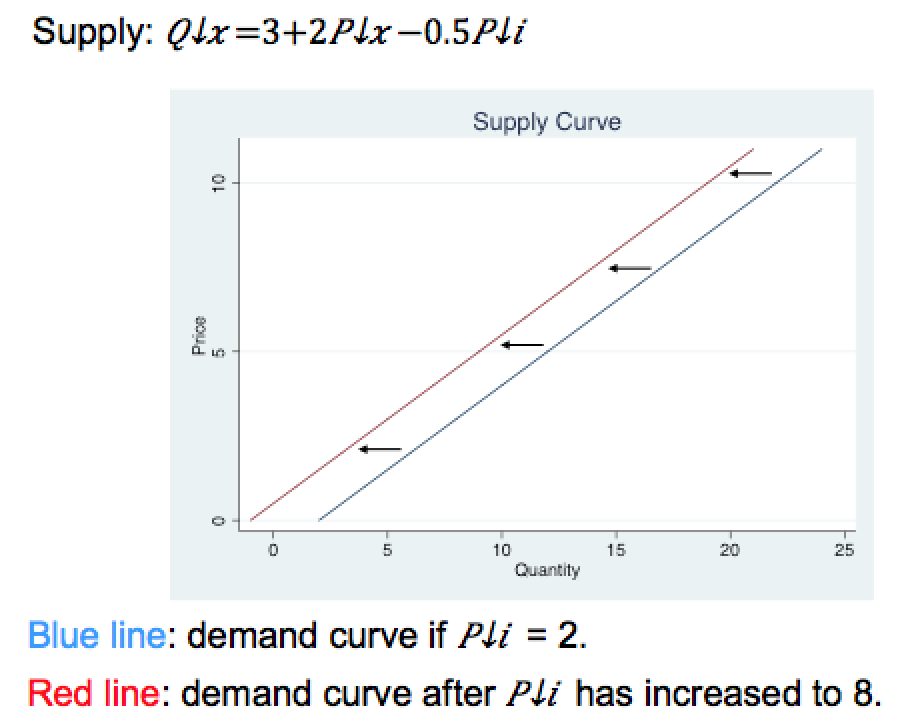
The Supply Curve - Math

The supply curve can be expressed as a mathematical function. For example:

Market Equilibrium

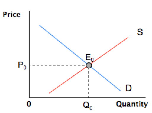
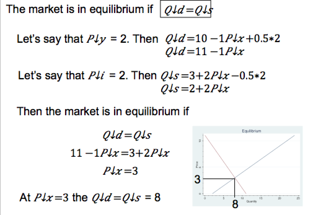
Market equilibrium is at E(0) where quantity demanded equals quantity supplied.

At a price of P(0) the quantity of Q(0) will be traded.

At P(0)Q(0) neither buyers nor suppliers want to change their behaviour, ceteris paribus.

Equi - equal + libra - balance

Equilibrium is point, or situation, of balance.

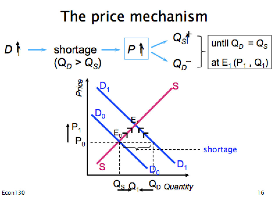
Example: A Shift in Demand

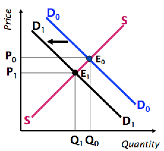
If the price of a substitute good decreases... less will be demanded at each price.

The demand curve shifts from D(0)D(0) to D(1)D(1).

If price stayed at P(0) there would be excess supply.

So the market moves to a new equilibrium at E(1).

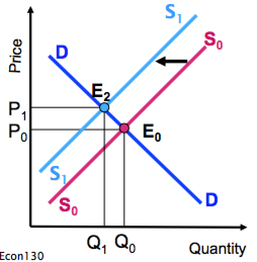
Example: A Shift in Supply

Suppose safety regulations are tightened, which prevents certain technologies from being used.

The supply curve shifts to S(1)S(1).

If price stayed at P(0) there would be a shortage.

So the market moves to a new equilibrium at E(2).

Markets and the Disequilibrium (1)

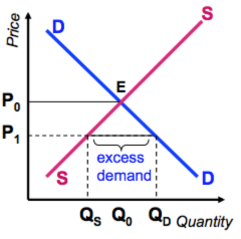
If price were below P(0) there would be a shortage.

Consumers wish to purchase more than producers wish to supply at P(1).

This is also called excess demand (Q(d)>Q(s))

Markets and Disequilibrium (2)

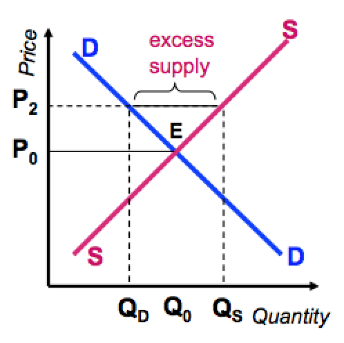
If price were above P(0) there would be a surplus.

Producers wish to supply more than consumers wish to purchase at P(2).

This is called excess supply (Q(s)>Q(d))

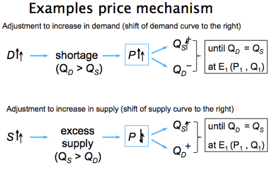
The Price Mechanism

Price is a central element in the free market process, bringing demand and supply into balance, or equilibrium.

- Price was Adam Smith's invisible hand: he proposed that prices could guide resources to their best use without central (state) coordination.

Partial Equilibrium Analysis

So far, we have analysed the market for a single good. In this market, the price of the good adjusts to equate Q(d) and Q(s) in equilibrium.

This is referred to as partial equilibrium analysis.

However, there are a number of other markets that might be affected by a change in one market.

A change in the market for sandwiches might affect, for example,

- the labour market and the bread market (input markets)

- the market for pizza (market substitute goods)

- the market for drinks (market for complement goods)

Typically that is okay, as the effects of one market on all others are often relatively insignificant.

General Equilibrium

General equilibrium (GE) analysis considers how the prices of all goods adjust (simultaneously) as as to "clear" (i.e. Q(d) = Q(s)) all markets.

- that is, GE describes a set of circumstances where all markets across the entire economy are in equilibrium at the same time.

GE analysis is also a starting point for macro-economics, which examines how the various markets in the economy interact together, and how a change in one market flows to the others.

Pareto Improvement

Pareto improvement is a change to a different allocation that makes at least one individual better off without making any other individual worse off.

A voluntary exchange leads to a Pareto improvement.

Example: selling a used car for $12,000

- buyer better off (other wouldn't have bought it)

- seller better off (other wouldn't have sold it)

Pareto Efficiency/Pareto Optimality

An allocation is Pareto efficient/optimal when no further Pareto improvements can be made.

Pareto efficiency/optimality is a state of allocation of resources in which it is impossible to make any one individual better off without making at least one individual worse off.

One can show that the allocation of resources in perfect competition is Pareto efficient.

This implies that:

- For a given allocation of goods, it is not possible to reallocate these goods amongst households to make someone better off without making someone else worse off

- It is not possible to change firms' production plans so as to produce more of one output, without producing less of another output.

- It is not possible to change the production mix (produce more of one good and less of another), so that the resulting output can make someone better off without making someone else worse off.

Perfect Competition vs Real Markets

In perfect competition, allocation is Pareto efficient.

However, real markets differ from perfect competition and therefore real markets can be inefficient.

When resources are allocated inefficiently or misallocated we have a market failure.

Reasons for Market Failures

Reasons for market failures include:

- Imperfect competition

- Public goods

- Externalities

- Imperfect information

Externalities

An externality is a cost or benefit imposed or bestowed on an individual or a group is outside, or external to, the transaction.

Examples:

- Improving your house yard (positive externally)

Neighbours benefit from it, but were not involved.

- Firm pollutes river to save costs (negative externality)

People living in the area suffer from it, but were not involved

Externalities - Inefficiency

Externalities lead to inefficiencies if they are not considered.

If producing a good creates costs for others (i.e., negative externalities) and these costs are ignored a profit-maximising firm would produce too much of this good.

Firms produce until P = MC, but MC do not include the cost imposed on others.

Government Intervention

Market failure might call for government intervention.

Government can intervene by imposing taxes or regulations.

In the pollution example, government can impose a tax for pollution or simply forbid it.

However, government intervention might generate more inefficiencies that it cures.