Dimensionality reduction and Visualization:

What is Dimensionality reduction?

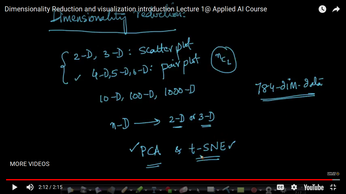
We realize that we can visualize data in 2-D or 3-D using a simple scatter plot and for 4-D,5-D and even 6-D, we use pair plot to sense how data is. Note: If we have to visualize our n-D data in pair plot then it can be done using nC2 scatter plots. So, pair plot will not work if n increases. There are 2 ways to reduce the dimensions to 2-D or 3-D. 1. PCA (old technique) 2. t-SNE (new)

Row Vector and Column Vector

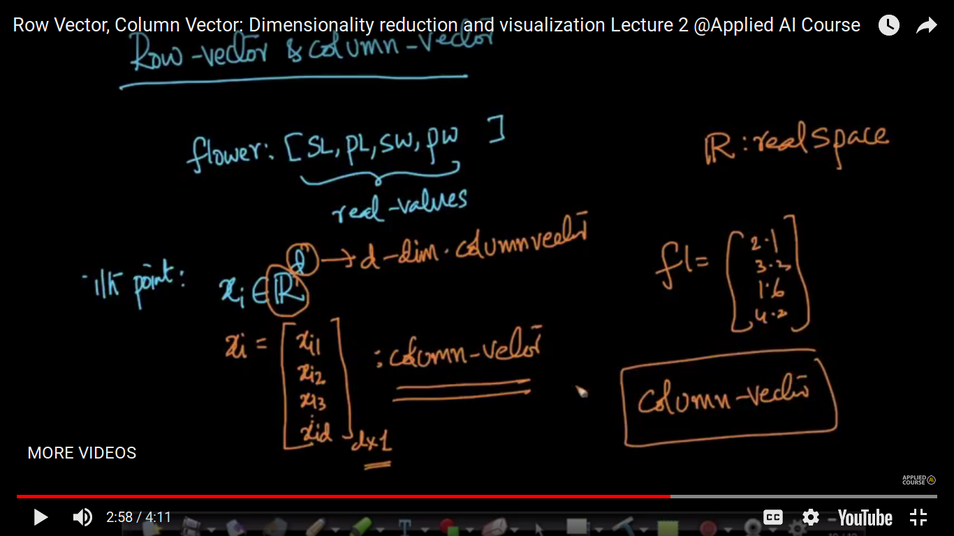
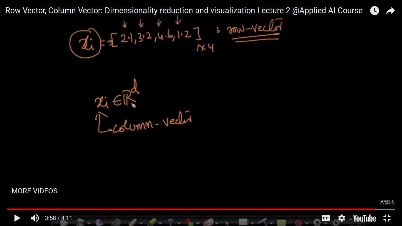
R - real space or real number or real values. If you are not told to be what kind of vector is, the default vector to be chosen is Column Vector If it specifies xi E R^d, then it is supposed to be a column vector.

How to represent a data set?

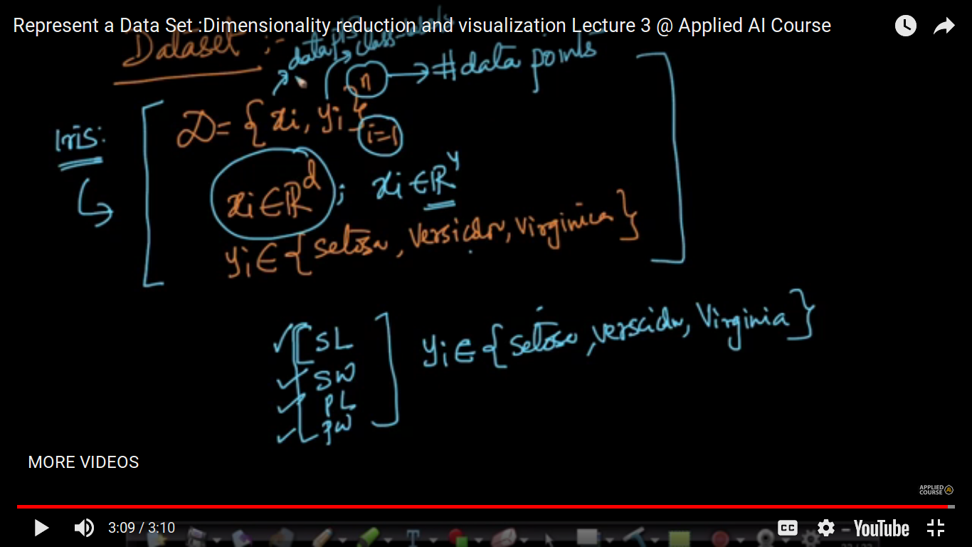
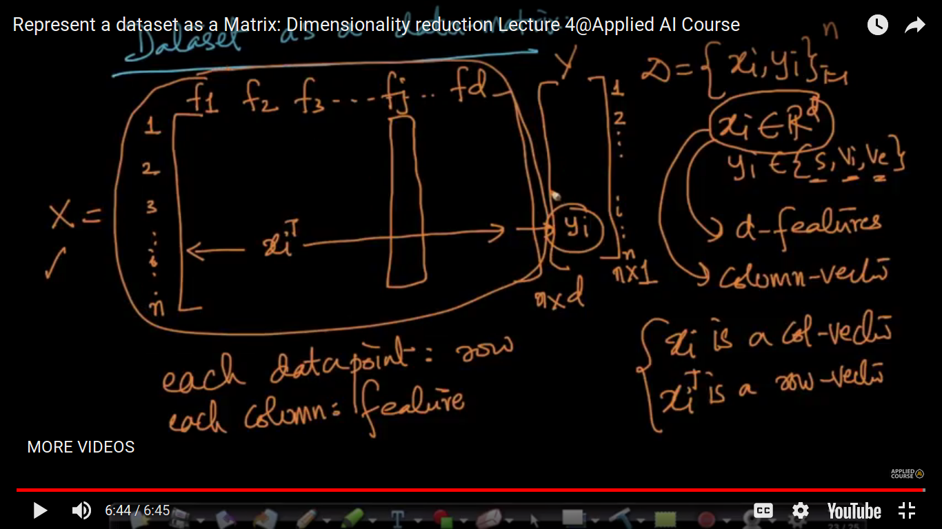
Yi may assume a real value or maybe something else i.e not always having a real value. D - Dataset D = { (xi, yi) }(1,n) read as Dataset D is a collection of data points xi and class labels yi and I have n such data points and each data point xi belongs to R^d(Example - R^4  where n=4 in IRIS dataset i.e a 4-D vector which contains sepal-length,sepal-width,petal-length,petal-width and yi belongs to 3 types of flower i.e Setosa, Versicolor and Virginica)   So, this is one way of representing a dataset but it may be many others.

How to represent a dataset as a Matrix

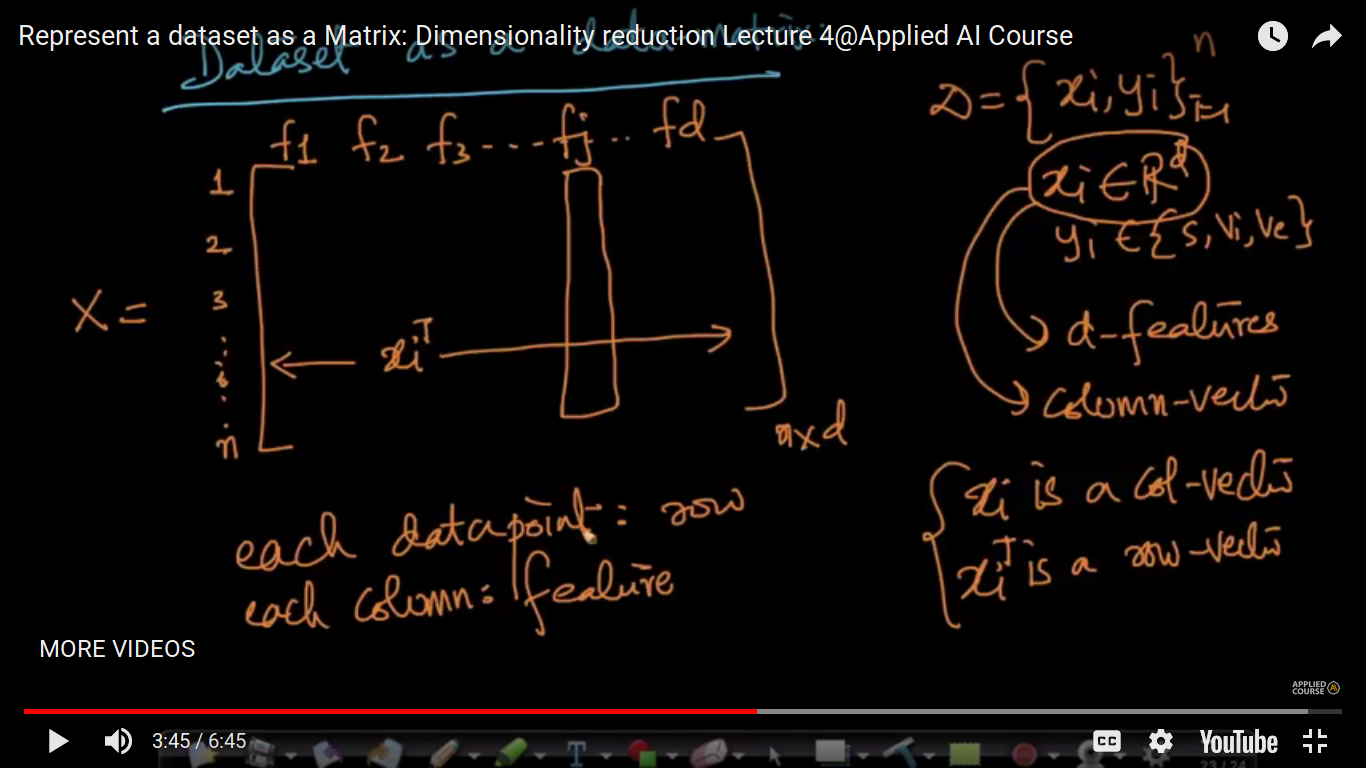
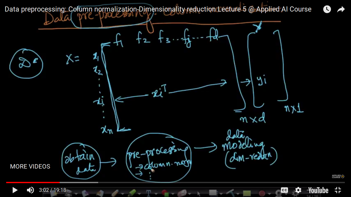
This is one of the ways of representing a dataset. Each column represents a feature and each row represent a  data point. But we have defined data point as xi E R^d i.e by default a column vector. So, we have to take transpose to represent a data point as a row vector.

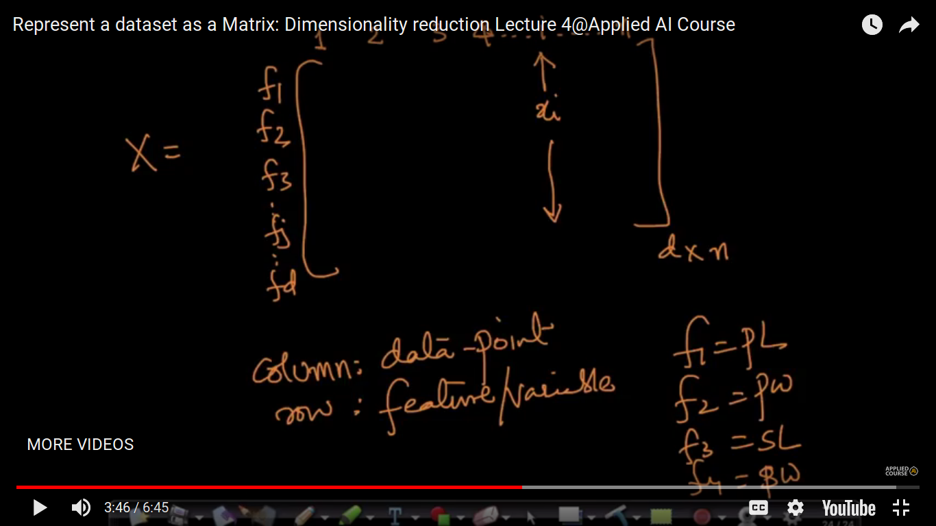
A lot of research papers represent below format. But both are valid ways of representation Because by default xi is a column vector so, they tackled in that way without converting xi to column vector by taking transpose. Or above method is valid because it more look likes a tabular approach. So, there is no right or wrong approach.

Data Preprocessing: Feature Normalisation

Data Preprocessing means that some type of mathematical operation and transformation on the data itself before we go for other more complex data transformation. We wanted to do dimensionality reduction so as to visualize our data more efficiently. So, we do data pre-processing means what type of operation you perform before you build models or pre-process our data so that it is in the form that is much easier for dimensionality reduction algorithm to use it. Therefore, we obtain data and do a further bunch of data pre-processing and then modeling of data. Note: Data Normalization is an extremely important task that we can perform over and over again.

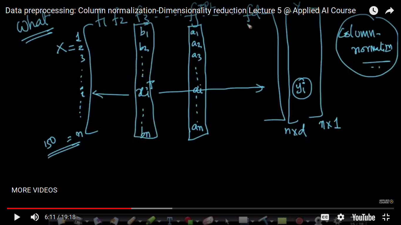
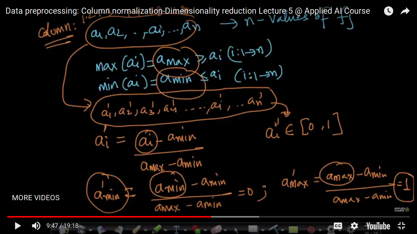
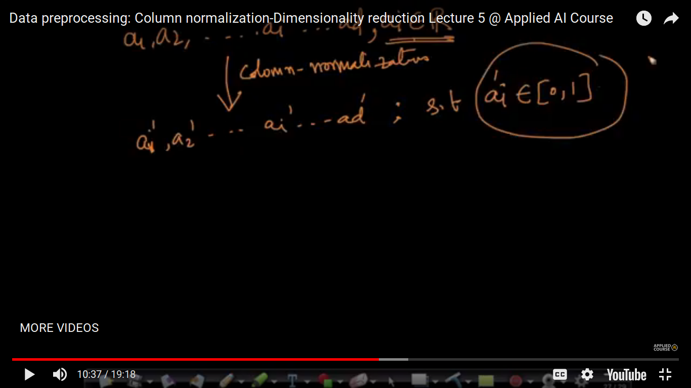
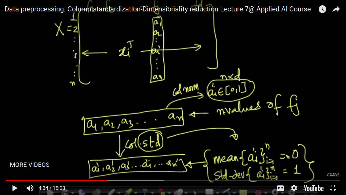
So, as a part of data pre-processing, one such operation that we performed is- 1. Column Normalisation   We are doing that because we want the value of a1' lies in between 0 and 1. So, in short, we transform the value of 'a'  i.e feature value lies in between 0 and 1 by using that formula.

So, below it's clear what we have to do? i.r transformation of ai to ai'

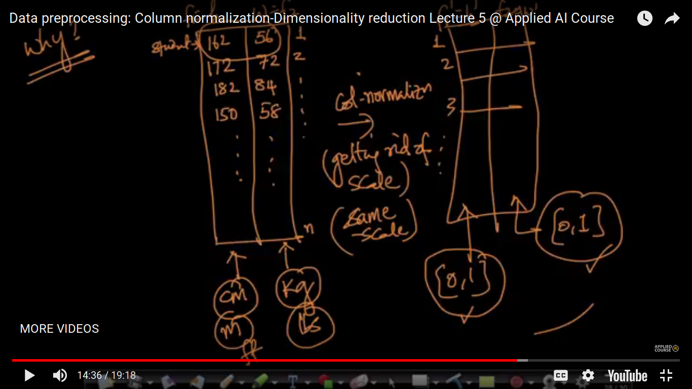
Now, why we are doing this? So, we know that real-world variables have many-many ways of collecting data. So, we say that whatever data we have collected, we don't care about the measurement scale(i.e cm, kg...feet) of data. Therefore, by doing this normalization I get my every feature into one standard format where all the values lie between 0 and 1. Note: On Normalization, this has become scale independent. So, scale becomes the problem when we are learning regression and classification techniques. Hence by normalization, we are putting all features on the same scale.

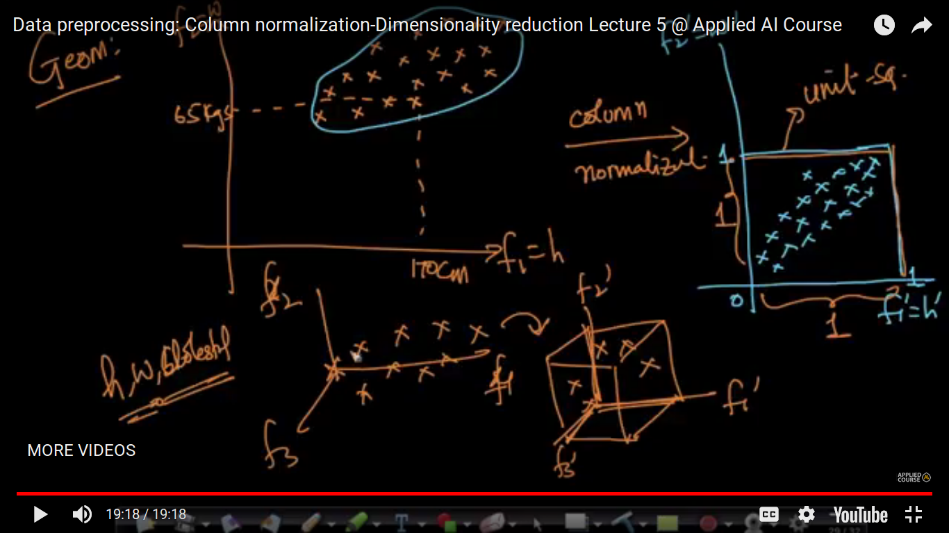
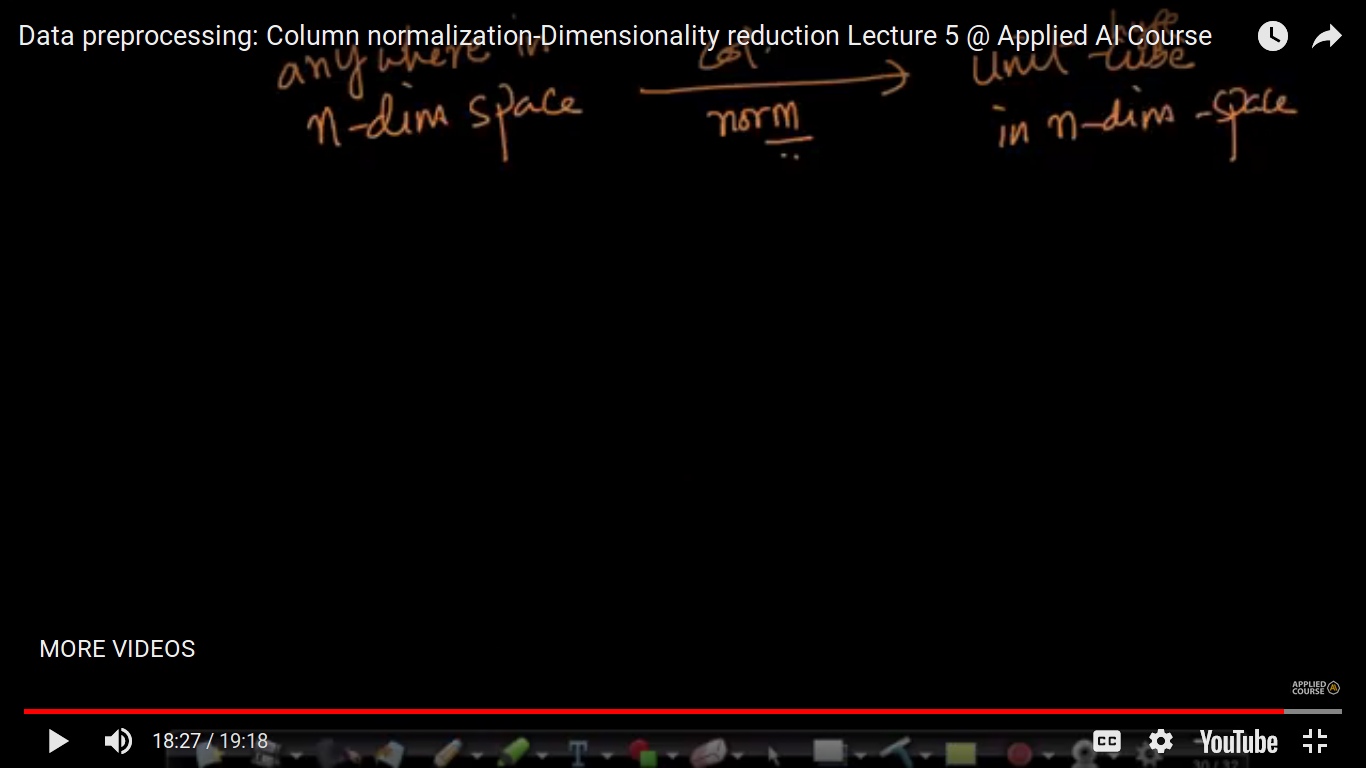
Now, let's understand Geometric Intuition or Interpretation: Here, we are squeezing our data between 0 and 1 i.e in a unit square without changing the relationships between data.

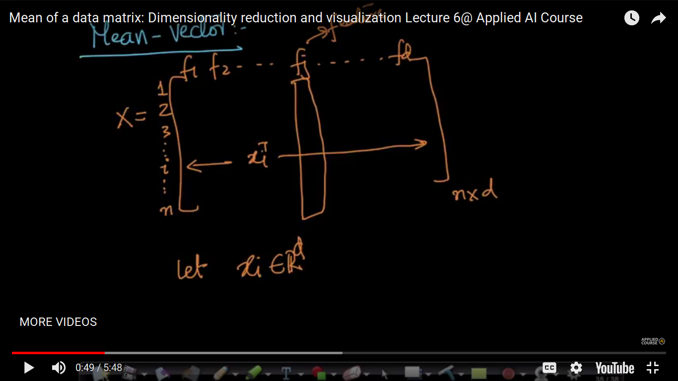
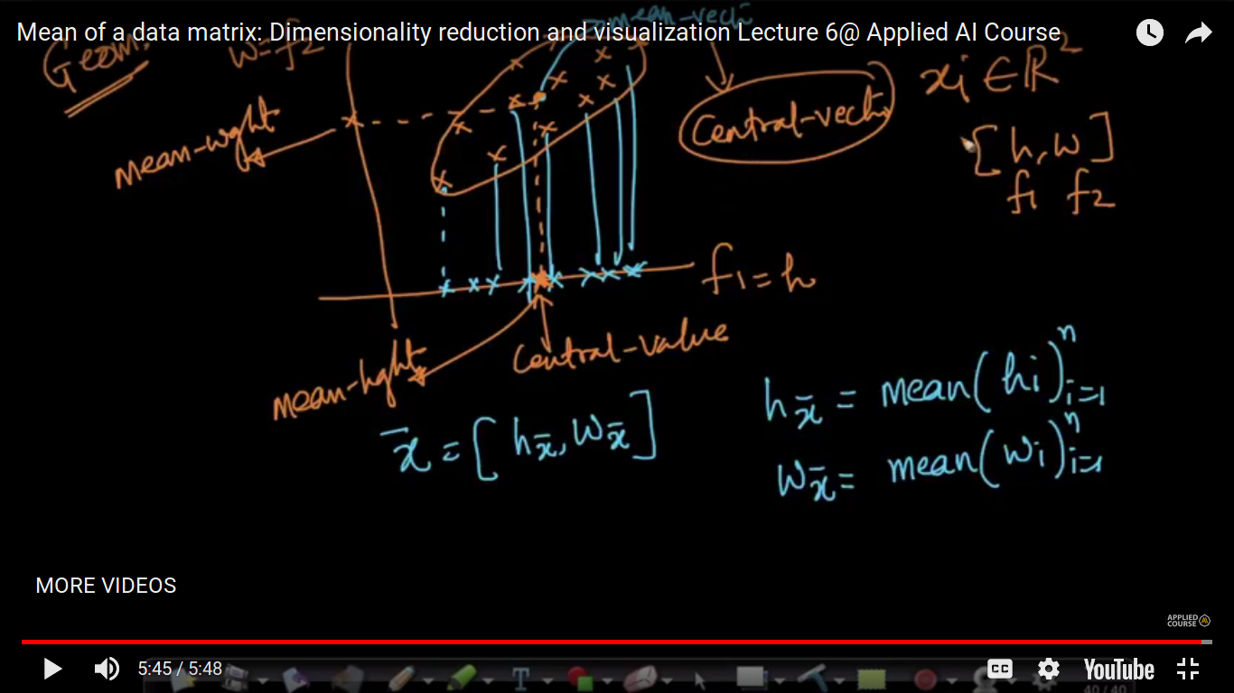
Mean of a data matrix

Here, xi is a vector and not scalar. Just like a scalar means, we can also define a mean vector.

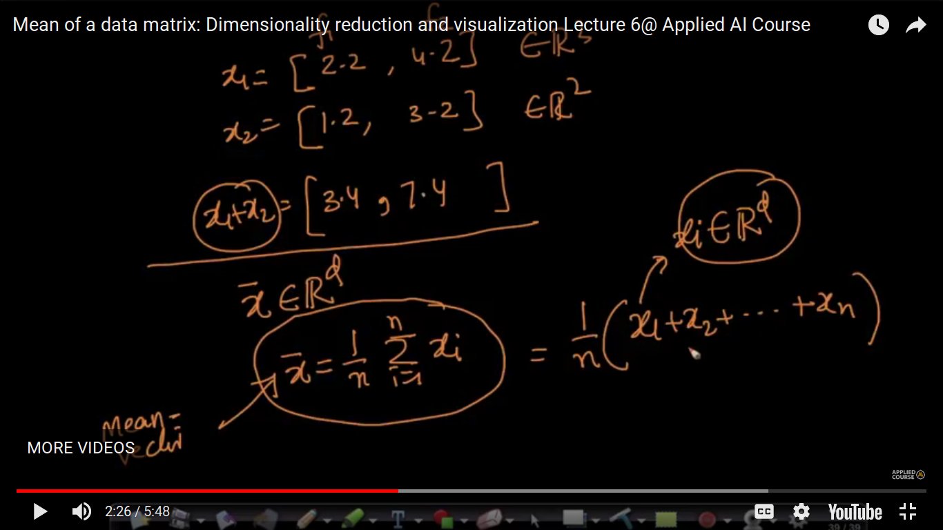
Just like mean is a central value for scalars, mean vector is a central value for the vectors.

What is the use of identifying a mean vector? Handling missing values by imputation which will be covered in Classification algorithms in various situations

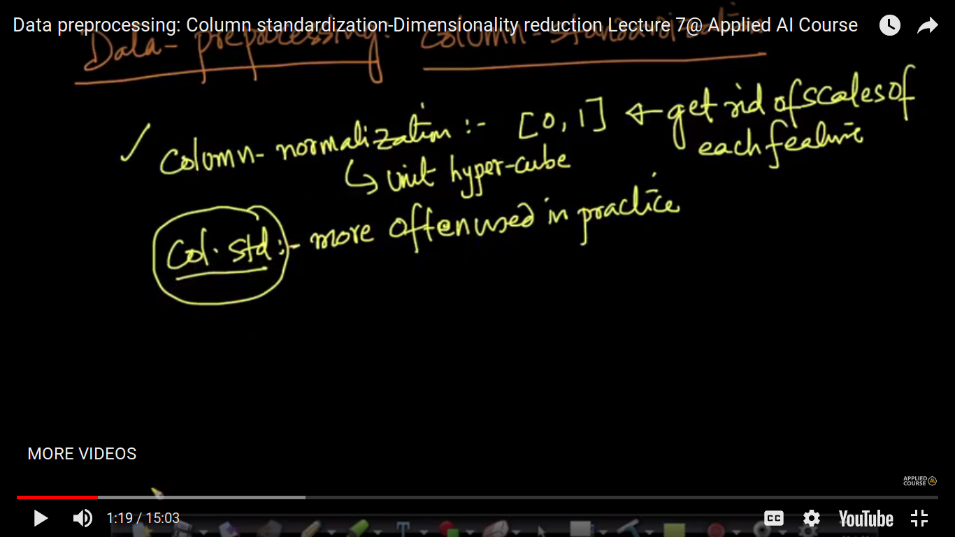
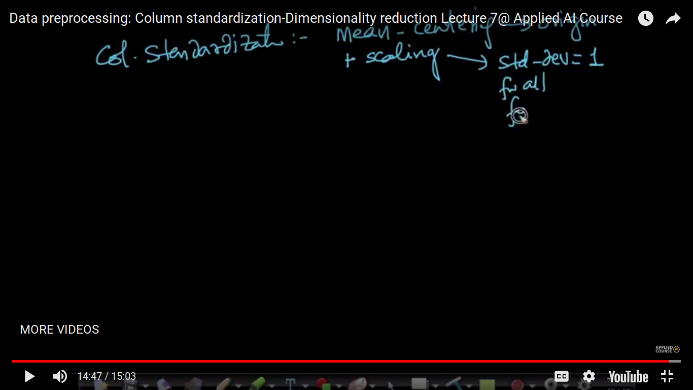
Data Preprocessing: Column Standardization

This is another technique of data pre-processing. And this is more often used than Column Normalization because it has a nice relationship to a Gaussian distribution.

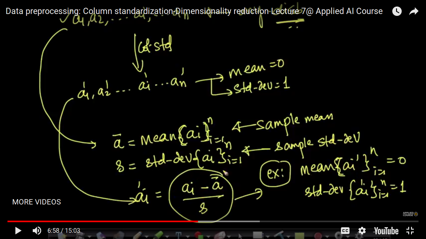
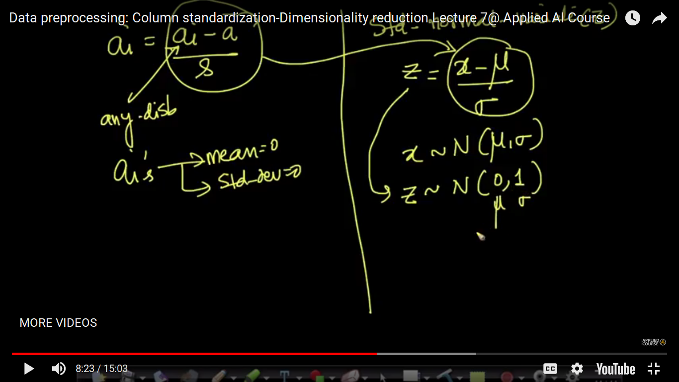
The idea of Column Normalization to squeeze data in between 0 and 1 is changed in the case of Column Standardization. Here, we convert ai to ai' in such a manner that the mean of ai' is zero and its standard deviation is 1. So, we can say that it is also one of the technique to get rid of the scale.

The formula of ai' is such a way that the overall mean of all the values of ai' is zero.

Why does it use Geometrically? Here, on column standardization, I am squeezing the data points so that its standard deviation on each of the axis is 1. So, I am squeezing or expanding the data points in such a manner its std deviation is 1. Example - If initially, the std deviation is sigma=0.5, then we have to expand and it's greater then 1, then we have to squeeze.

In short, we are moving the mean vector to the origin and we squeeze if std deviation is greater than 1 and expand if less than 1.

Note - Q&A After column standardization, all the values are transformed in such a way that the mean of all the transformed values becomes ‘0’ and the standard deviation of all the transformed values will become ‘1’. All the standardized values should be accommodated within 1 standard deviation(sigma=1). Squishing of Data Points after Column Standardization: If “sigma(before standardization operation) > 1, then all the transformed data points will be accommodated within a distance of ‘1’ from the origin. That is the standard deviation value decreases after Standardization. This is called “Squishing/Compression of data points”. Expansion of Data Points after Column Standardization: If “sigma(before standardization) < 1, then all the transformed data points will be accommodated within a distance of '1' from the origin. That is the standard deviation value increases after Standardization. This is called "Expansion of data points".

when we standardize it, it follows n(0,1) then why are we saying that it is not Gaussian distribution?? If the original random variable follows the Gaussian distribution then after standardization also it follows the gaussian otherwise not. https://soundcloud.com/applied-ai-course/standardization-vs https://www.appliedaicourse.com/course/applied-ai-course-online/lessons/local-outlier-factora/

what are the cases in which we should do normalization instead of standardization? Answer: Standardization (using mean and std-dev) is better when we have outliers as outliers will have large negative or positive values while inliers will have values around 0. Normalization (using min and max) in the case of data with outliers could result in outliers having values closer to 0 and 1 and most inliers concentrated in a small band of values. Normalization is better if we want all resulting values in the interval [0,1] as Standardization can result in any value, both positive and negative.

NORMALIZATION: Data normalization is the process of rescaling one or more features to the range of 0 to 1. This means that the largest value for each feature is 1 and the smallest value is 0. Normalization is a good technique to use when you do not know the distribution of your data or when you know the distribution is not Gaussian (a bell curve). Normalization is useful when your data has varying scales and the algorithm you are using does not make assumptions about the distribution of your data Standardization: Data standardization is the process of rescaling one or more features so that they have a mean value of 0 and a standard deviation of 1. Standardization assumes that your data has a Gaussian (bell curve) distribution. This does not strictly have to be true, but the technique is more effective if your feature distribution is Gaussian. Standardization is useful when your data has varying scales and the algorithm you are using does make assumptions about your data having a Gaussian distribution

why standardization is more effective if the distribution is Gaussian? Column standardization is more effective when the underlying distribution is Gaussian with say mean=mu and std-dev=sigma. This is due to the fact that when you normalize such a feature, you get the new feature to be of N(0,1) distribution. This is an ideal distribution with lots of ML, Stats and Optimization techniques assuming a Gaussian distribution to make the proofs work beautifully. You will be able to appreciate it better when you learn logistic regression and it’s probabilistic interpretation (Gaussian Naive Bayes) later in this course. That doesn’t mean standardization is not good for no-gaussian distributed features. It still results in a new feature with a mean of 0 and variance of 1, but not N(0,1) distribution. In practice, we perform standardization irrespective of the underlying feature distribution. But the mathematical proofs are well suited when the distribution in Gassian. That’s all.

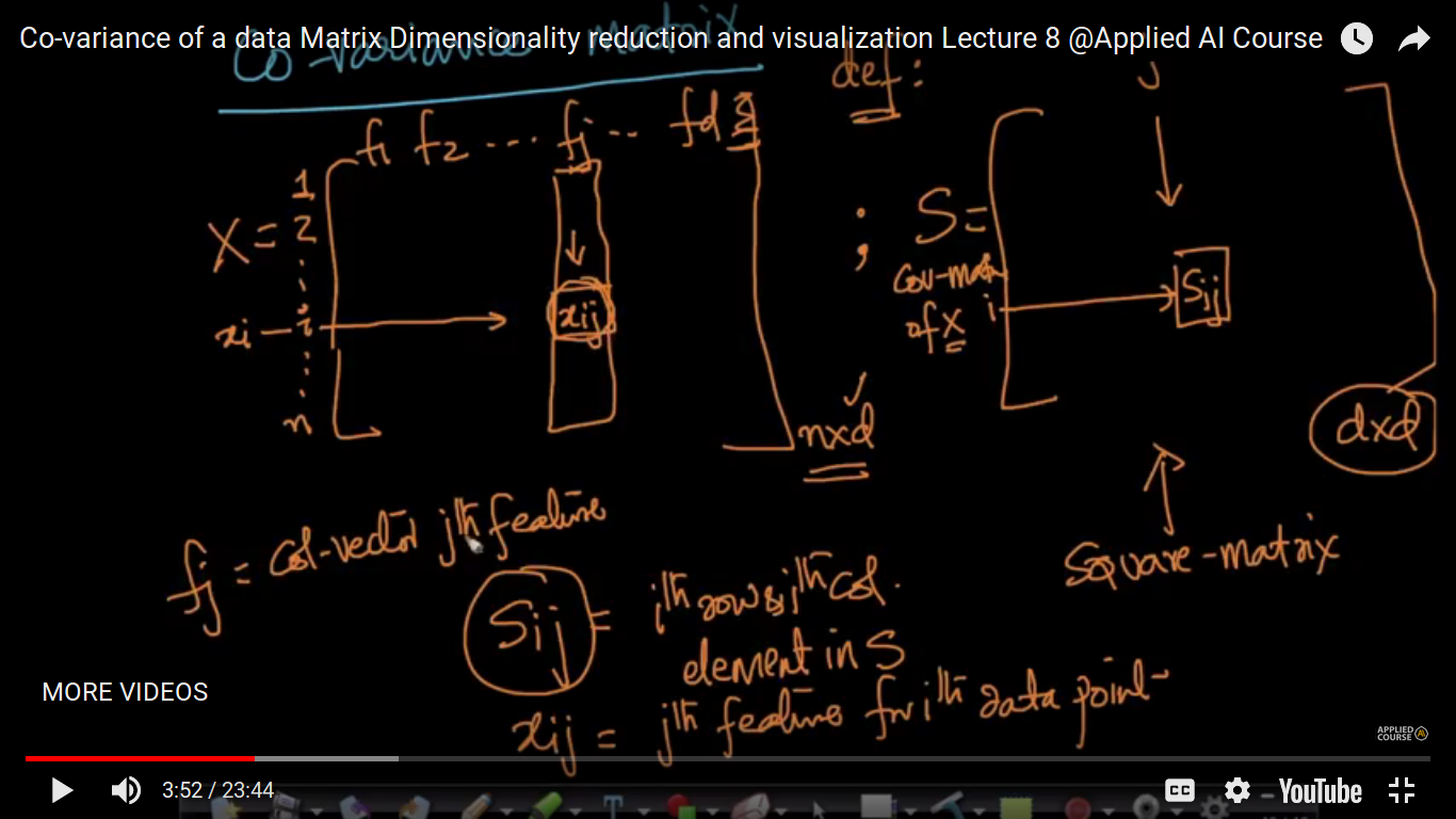
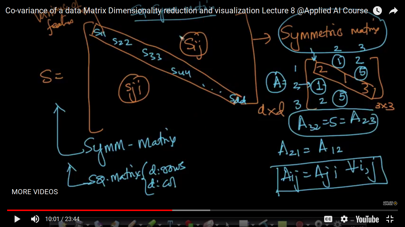
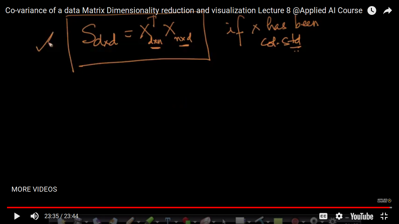
Co-variance of a Data Matrix

Here, X is a data Matrix and S is a Co-variance matrix of X.

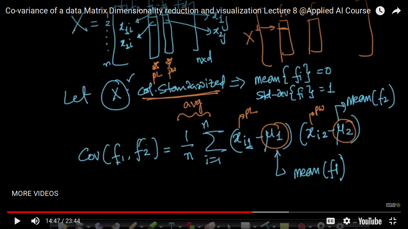
we saw its geometric interpretation when we are discussing the correlation coefficient, the Pearson Correlation Coefficient, Spearson etc. So, here we are discussing the formula and properties of CoVariance.

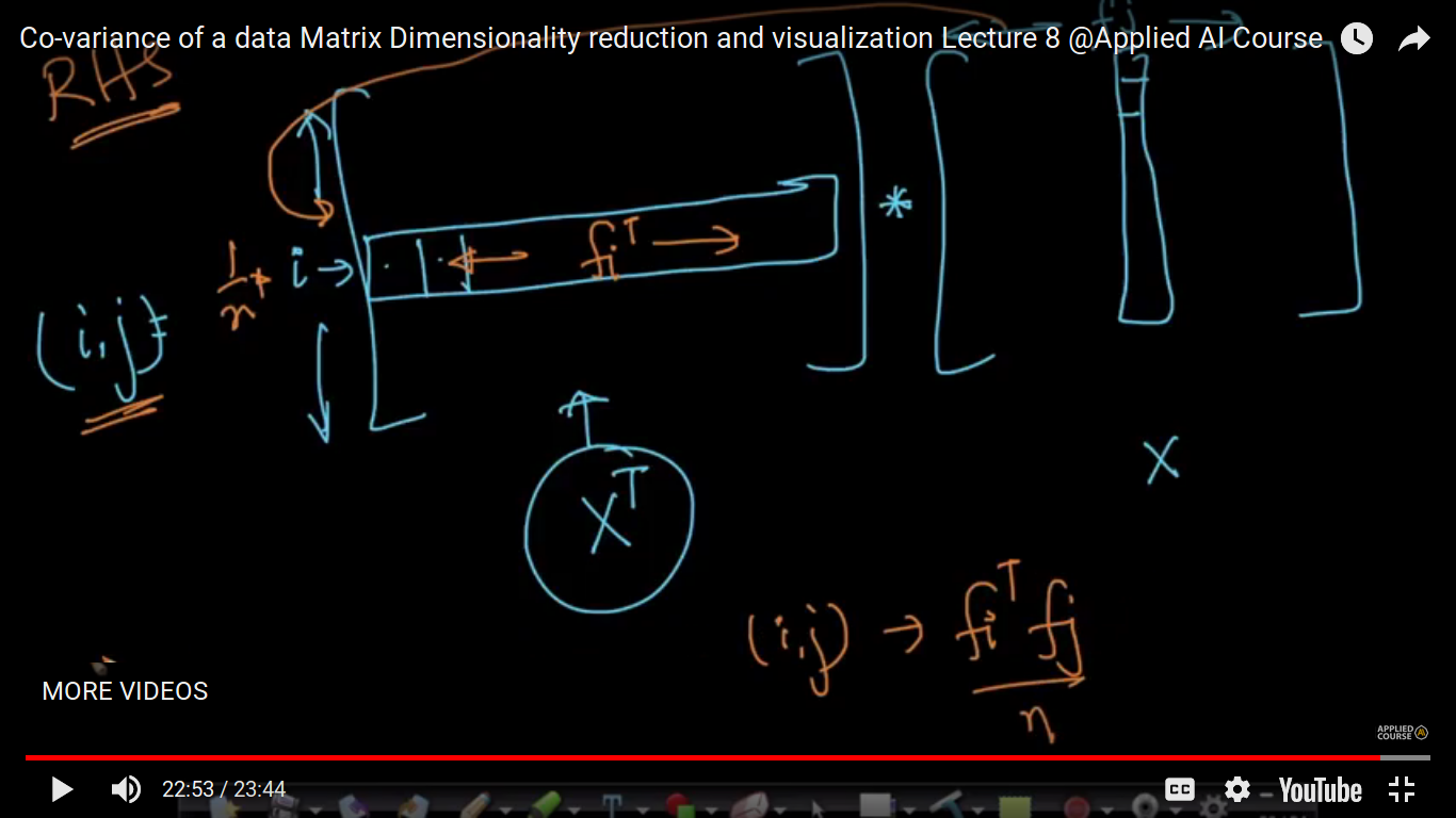
We just define its definition and now we will see why it is useful.

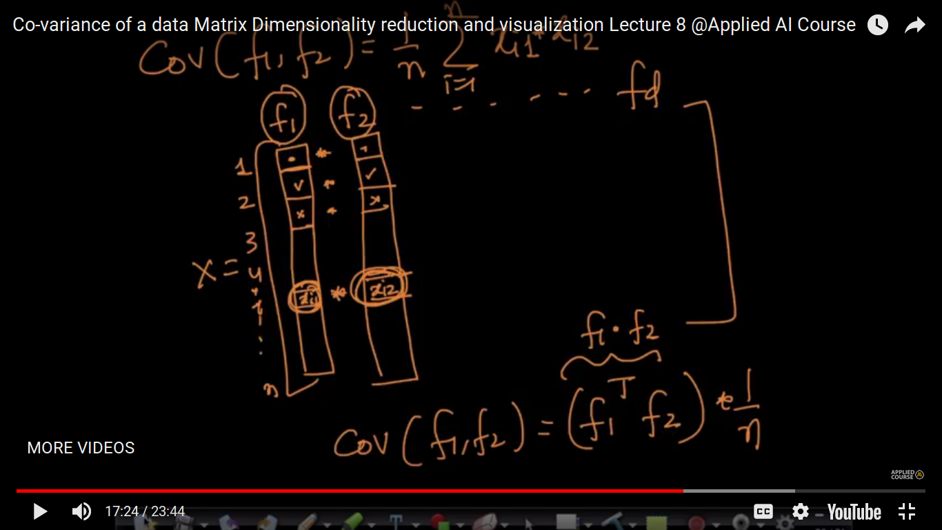
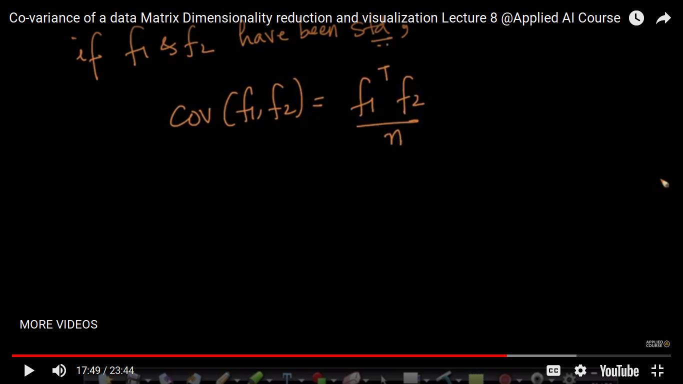
Here, we are taken f1^T * f2 as we are doing component-wise multiplication followed by addition and often it is the dot product of f1 and f2.

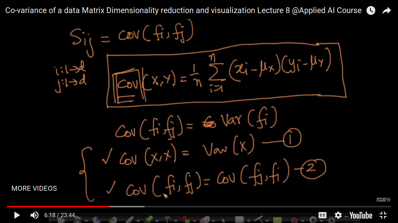
The above formula of the covariance matrix is extensively used when are doing a dimensionality reduction using PCA.

Note: Q&A 1. Given a Data matrix “X” of size (n*d) Then we will have a Cov-matrix “S” of size (d*d) that is an sqr matrix. So my question is if we simply create a (d*d) matrix of “X” features “d” then that would be called a covariance matrix? 2. Why are we calculating cov(fi, fj)? I actually understood that how it is calculating but not getting why it is being calculated? Is cov-matrix is made by calculating cov(fi,fj)??   1. No, you have to compute covariance of two random variables and keep it in matrix form. Let’s take the example of MNIST data, it has 784 dimensions, now compute covariance between every pair of features then store it in a matrix. 2. Covariance is a measure of how much two random variables vary together. It’s similar to variance, but where variance tells you how a single variable varies, covariance tells you how two variables vary together.

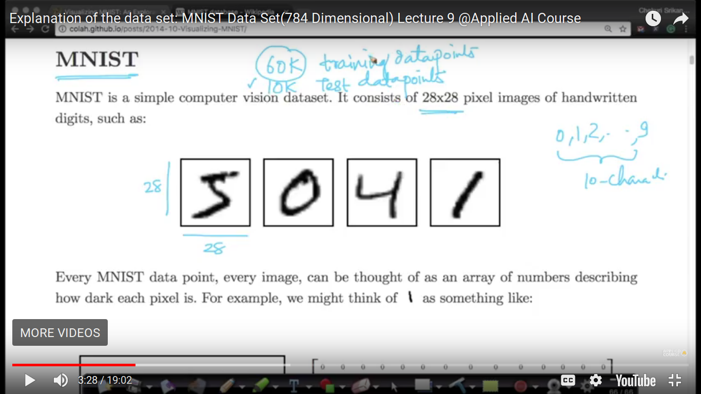
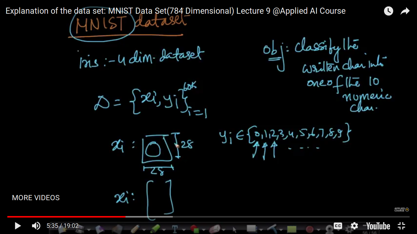
MNIST dataset (784 dimensional)

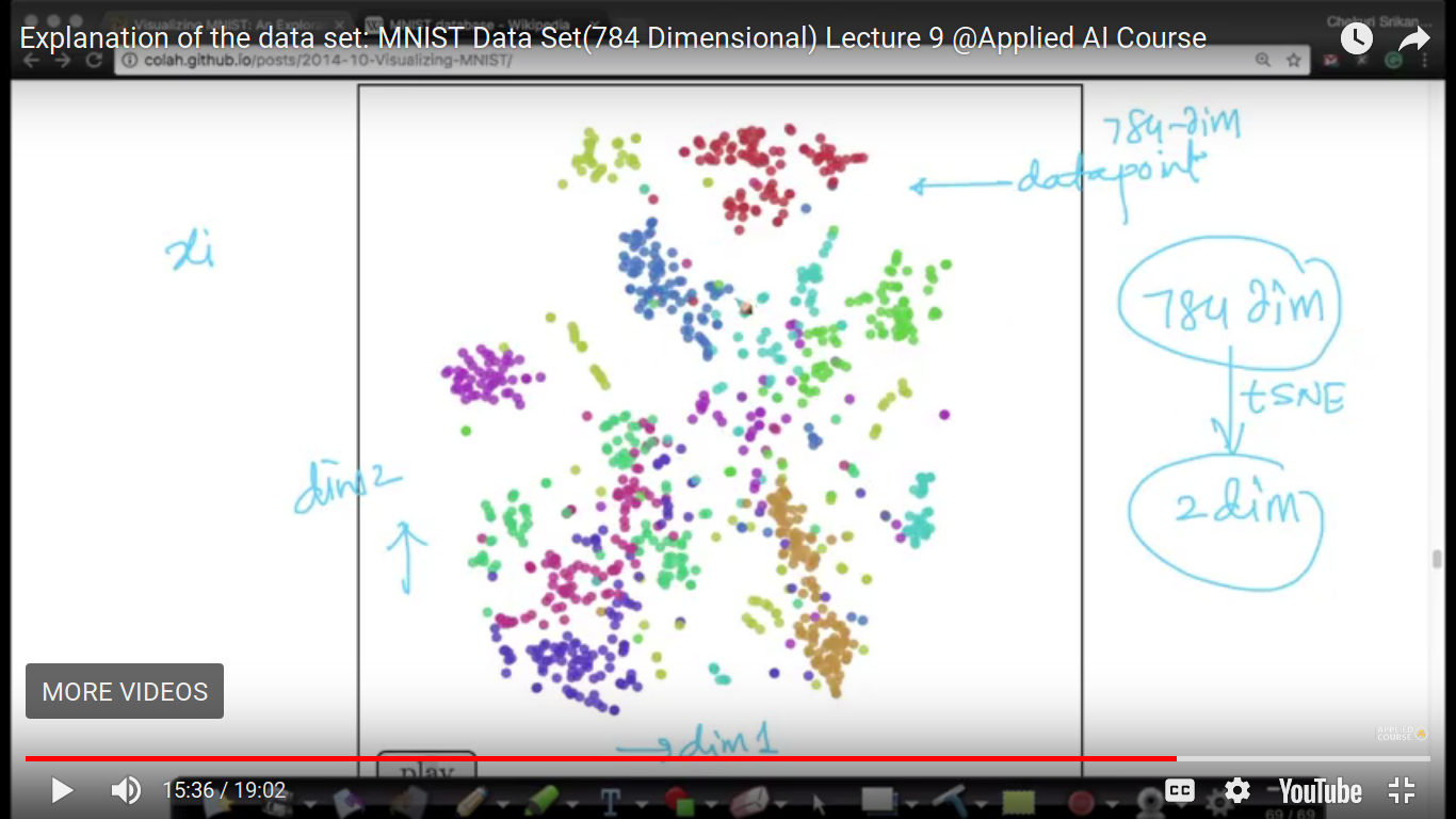
Since this chapter is all about visualizing high dimensional data just like a 4-D  IRIS dataset in Exploratory Data Analysis.al So, now we have MNIST dataset to visualize high dimensional dataset and dimensionality reduction. .link: colah.github.io Visualizing MNIST

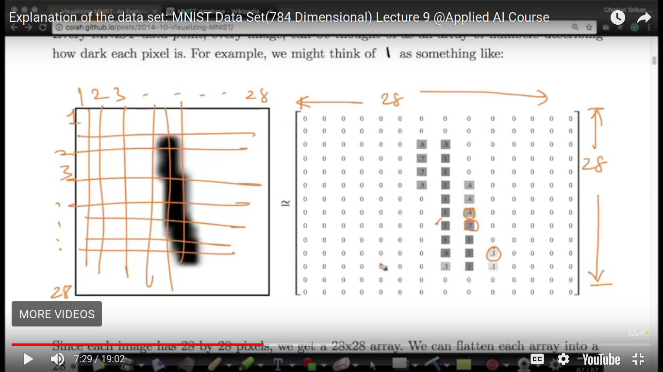
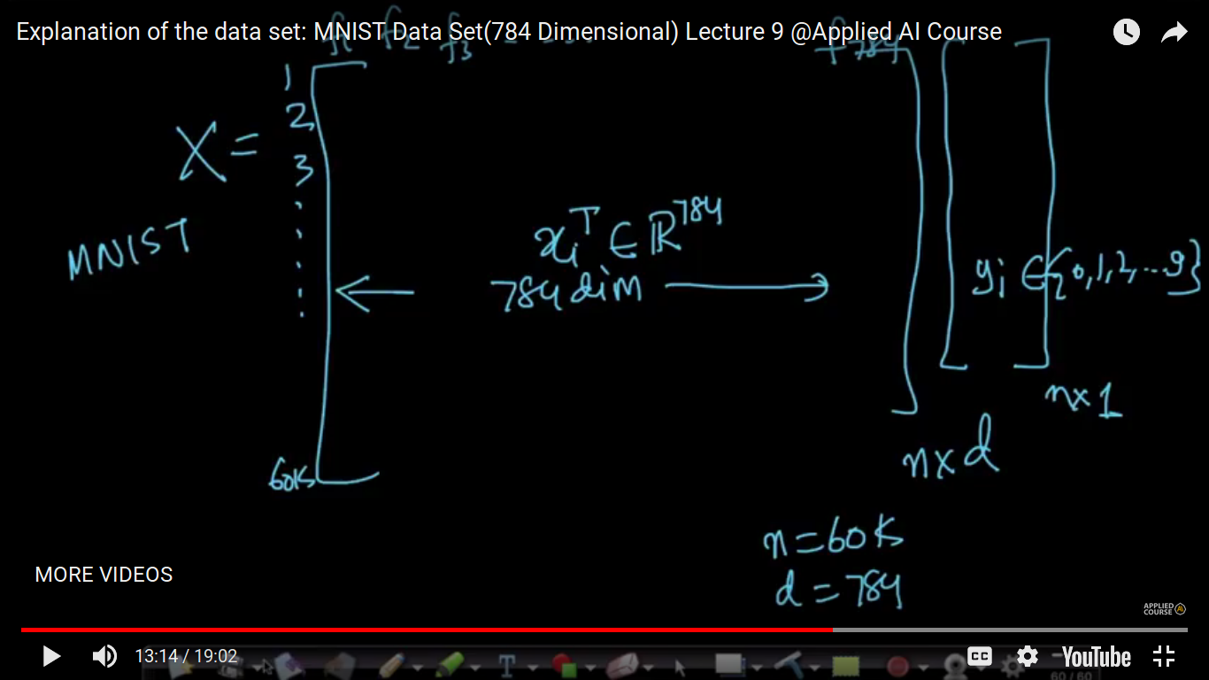
The MNIST dataset is a handwritten character and then take a photo of it. The pixels of the image is 28X28. Now, we have 60K training data points and 10K Test data points. So, we have to build a model using 60K training data points and test it on a 10K dataset. This terminology training and testing shall be covered up in Classification Algorithm.

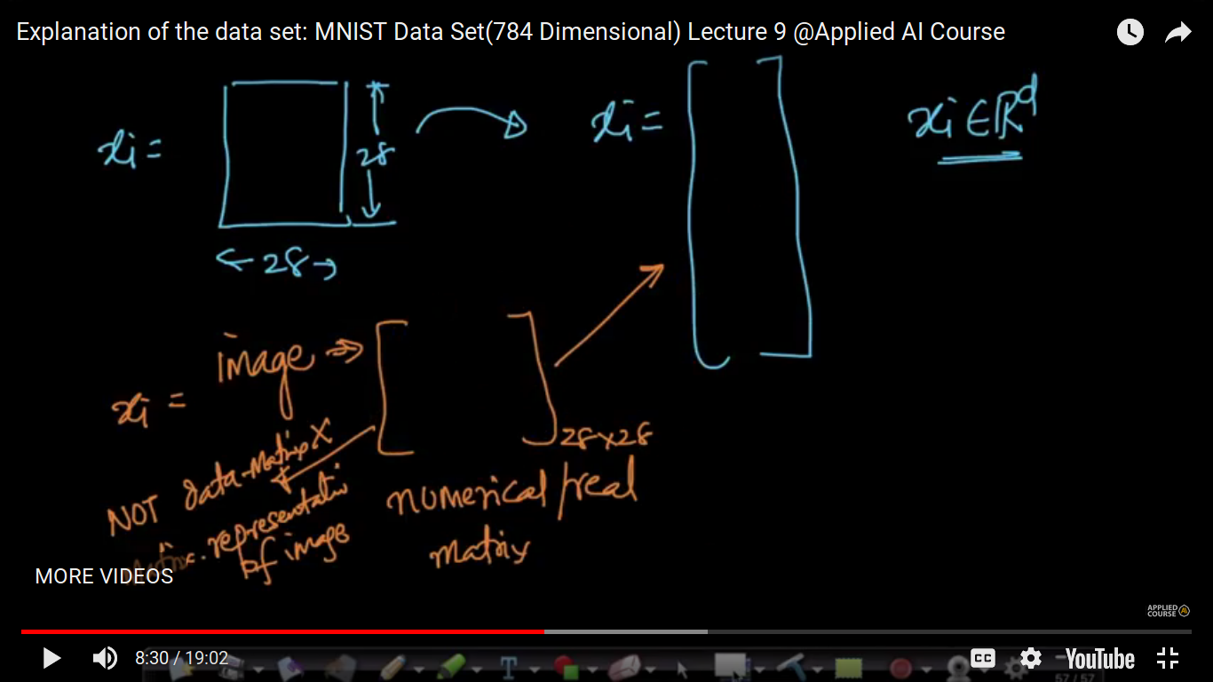
Here, we have an image which is converted into a numerical/real matrix. For Example -  White color is represented is '0', black color is represented as '1', grey is '4' etc That 28X28 matrix is not a data matrix, it's called a data point(xi). Now, let's see how we can convert that matrix of pixels into vector matrix.

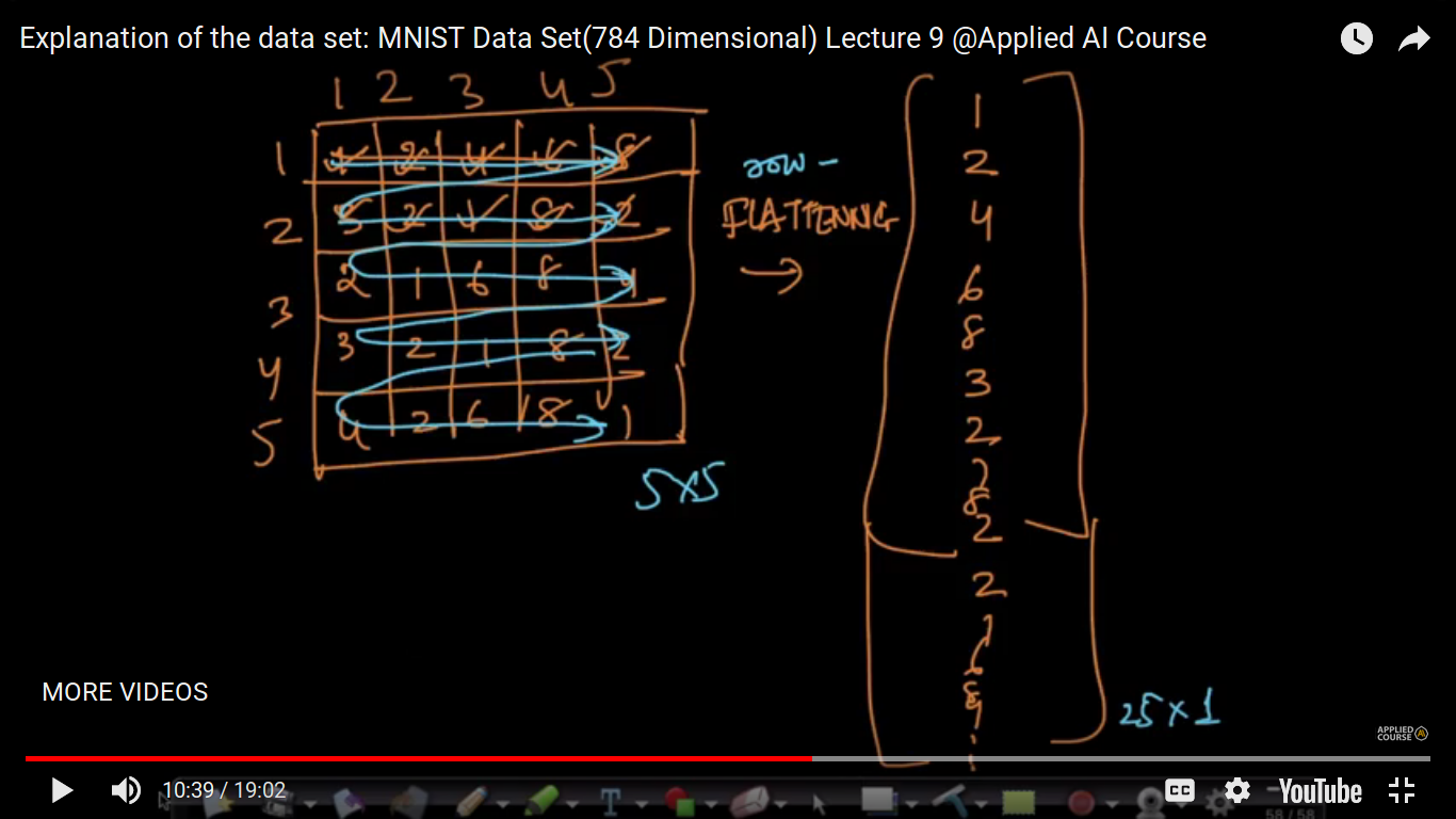
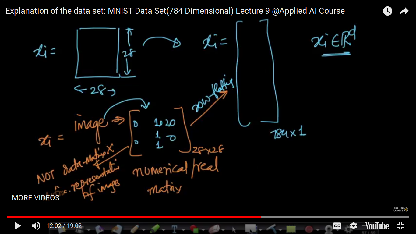
So, in order to do matrix representation of an image into a data matrix. Now, we will do Flattening i.e taking each row and write it on a column vector matrix. We can do both row flattening and column flattening.

Now, each data point is denoted by X and it is of a 784X784 matrix.

Code to Load MNIST Data Set

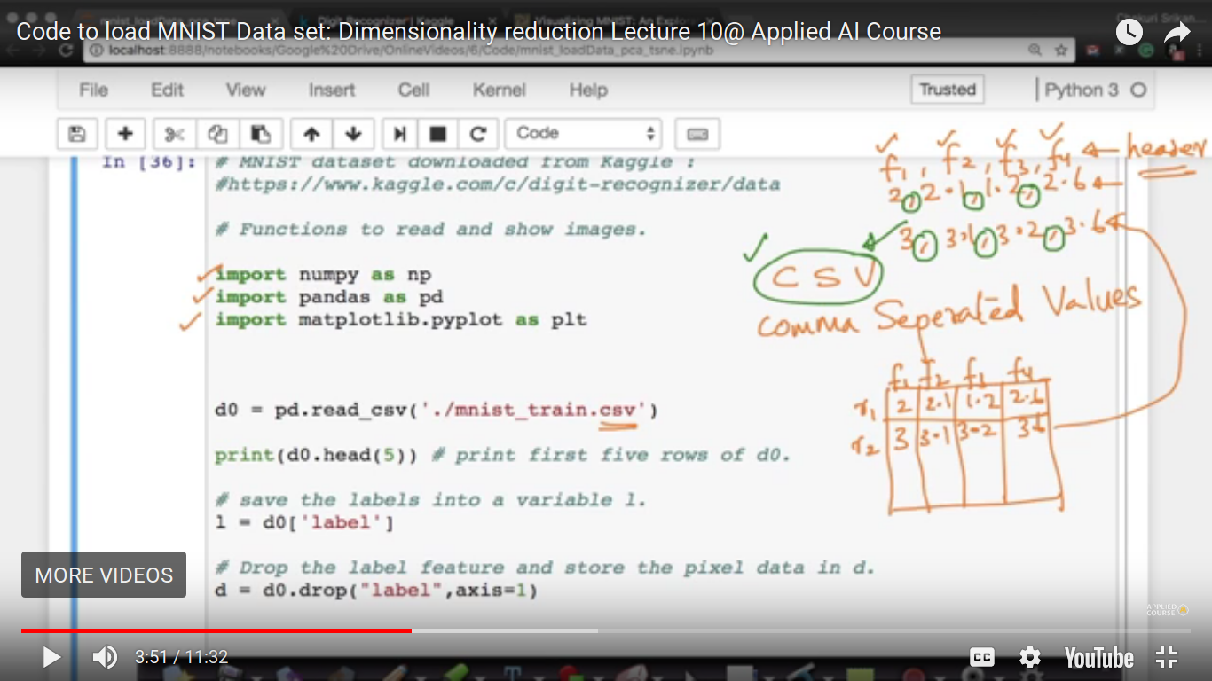
This involves the general Code Explanation. This is also ipython file attached to that folder.  So, rest of the code can be referred to that location.