Probability & Statistics
|
|
Created by Rohit Gurjar
almost 7 years ago
|
|
| 0 | ||
| 0 | ||
| 0 | ||
| 0 | ||
| 0 |
0 comments
There are no comments, be the first and leave one below:
Kernel Density Estimation
1. KDE is one way to smooth a histogram. Smoothed functions are easier to represent in functional form i.e., as f(x) as compared to non-smooth functions. Additionally, smooth functions represented as f(x) as easier to integrate. We need integration as CDF is an integration over PDF. Smooth functions represented in functional form are easier to manipulate to build more complex operators on the data.
2. KDE is used to obtain a PDF of an r.v. Histograms and PDFs inform of the density of data for each possible value an r.v takes. We have explained about PDFs and their interpretations in details in the above videos in EDA especially in this one: https://www.appliedaicourse.com/course/applied-ai-course-online/lessons/histogram-and-introduction-to-pdfprobability-density-function-1/
If we decrease the window size and increase the number of bins then the graph of PDF becomes zagged like structure
This is the kernel density gaussian kernels.
##
Yes, the variance for these Gaussian kernels is a parameter which we can tune based on our need for smoother or jagged PDFs. If we keep the variance very small, we get a very jagged PDf and if we keep it too wide, we get a useless and flat PDF. So, it is a tradeoff. In practice, most of the plotting libraries use rules-of-thumb or various algorithms to determine a reasonable variance.
For example in SciPy, the bandwidth parameter determines the variance of each kernel. There are many methods to determine the bandwidth parameter as per this function reference: https://docs.scipy.org/doc/scipy/reference/generated/scipy.stats.gaussian_kde.html
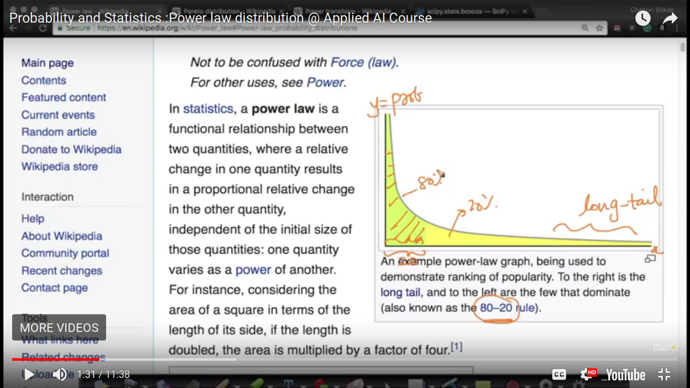
If X follows power law distribution, then it's called Pareto distribution
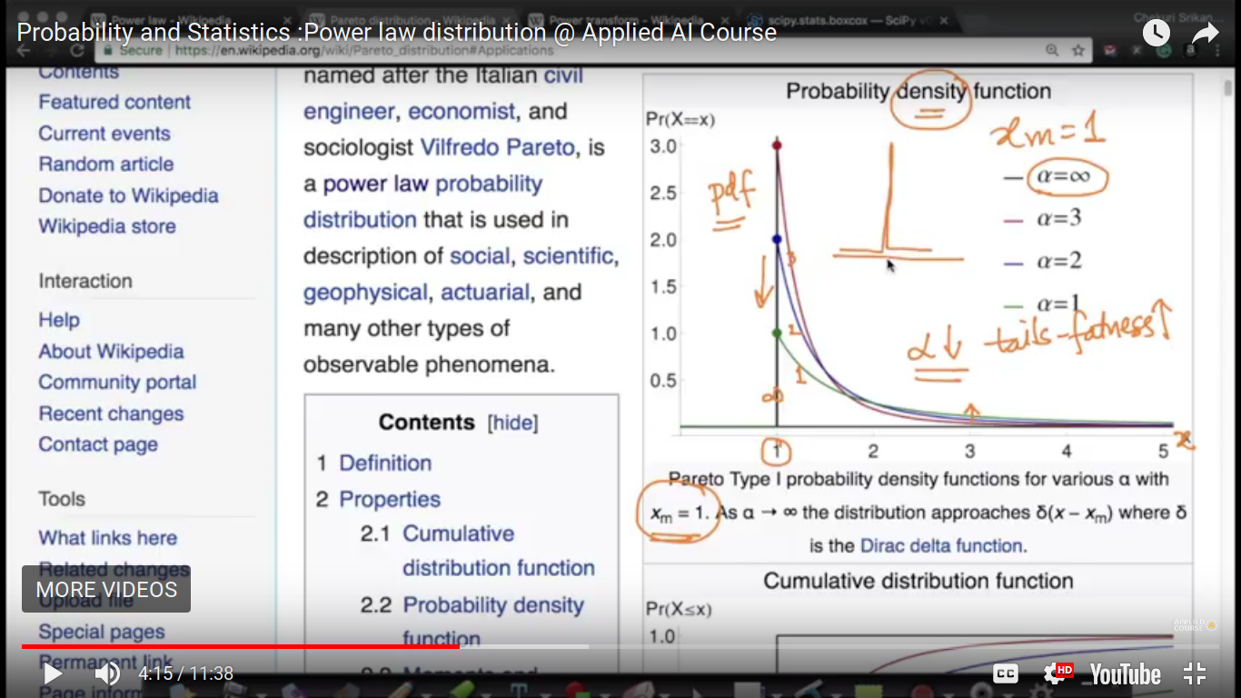
Dirac Delta Function - Everywhere else is zero but at one given value x=1, it attains peak.
When alpha tending to infinity then Dirac delta function condition occurs.
So, for Log Normal, it attains a peak value and then a fall off and for Perito distribution, it has a peak value and then slightly fall off.
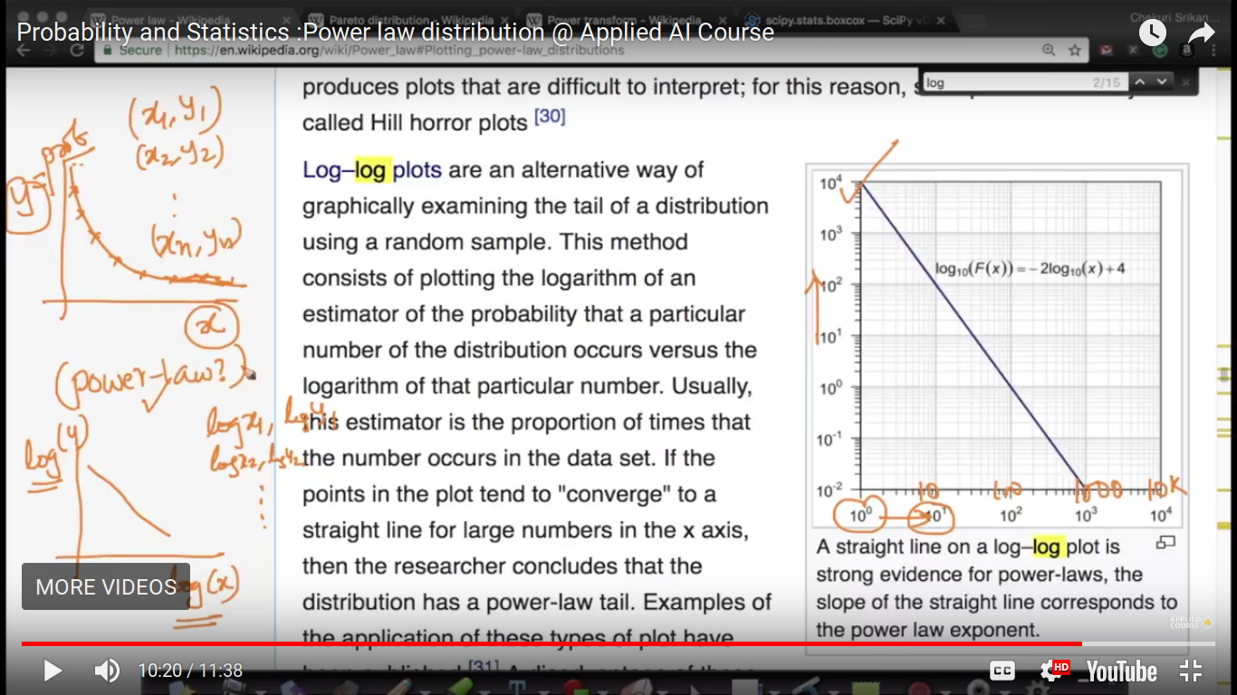
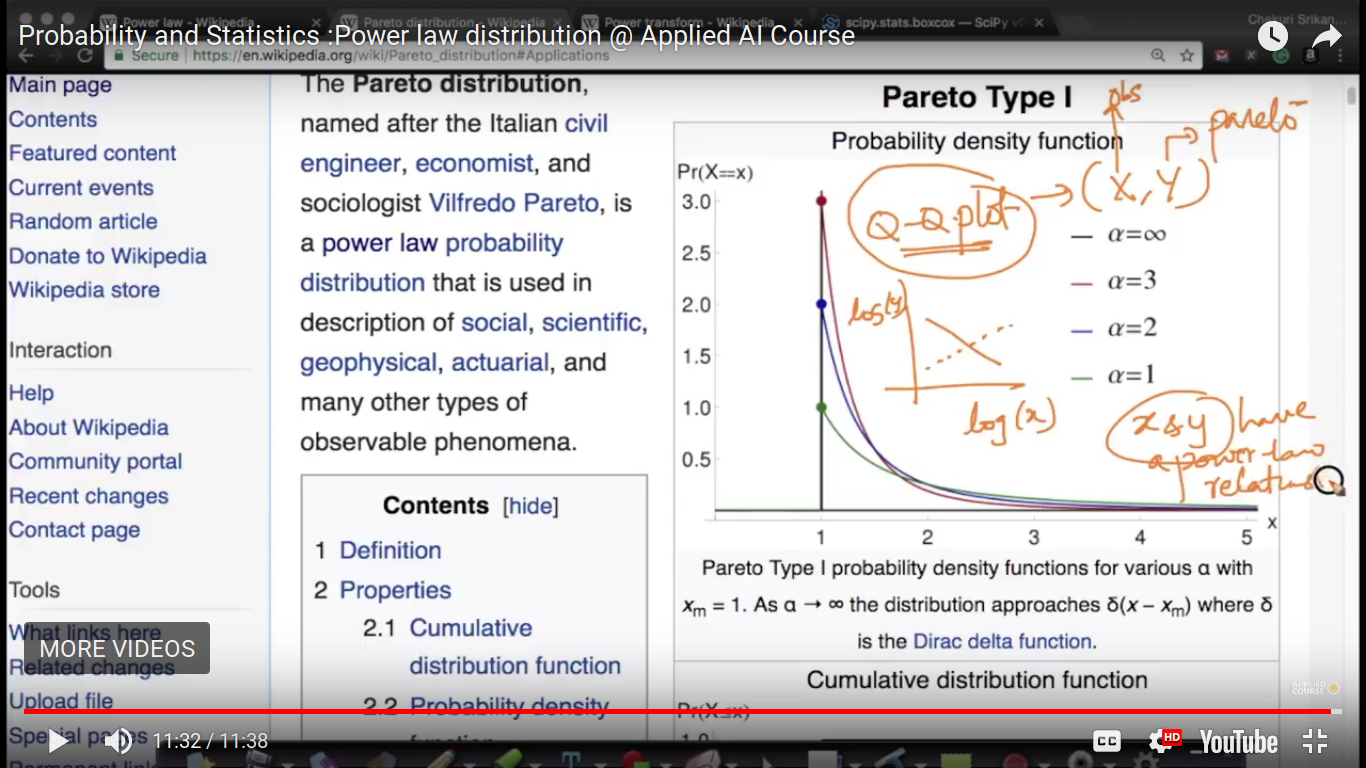
To predict X and Y have a power law relation, we can first find logX and logY and the draw Q-Q plot.