Probability & Statistics
|
|
Created by Rohit Gurjar
almost 7 years ago
|
|
| 0 | ||
| 0 | ||
| 0 | ||
| 0 | ||
| 0 |
0 comments
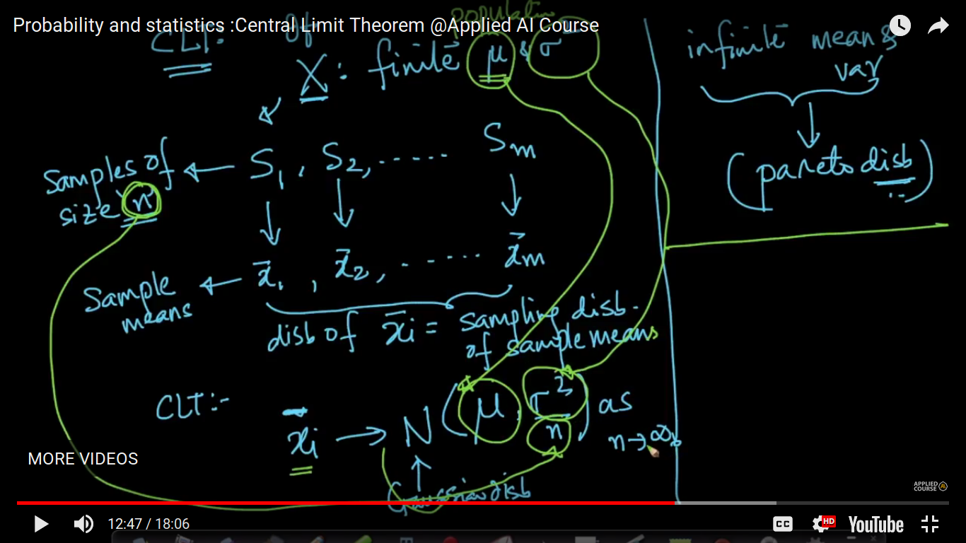
The central limit theorem states that if you have a population with mean μ and standard deviation σ and take sufficiently large random samples from the population with replacement, then the distribution of the sample means will be approximately normally distributed. This will hold true regardless of whether the source population is normal or skewed, provided the sample size is sufficiently large (usually n >= 30). If the population is normal, then the theorem holds true even for samples smaller than 30
Distribution implies PDF(Probability Distribution Function)
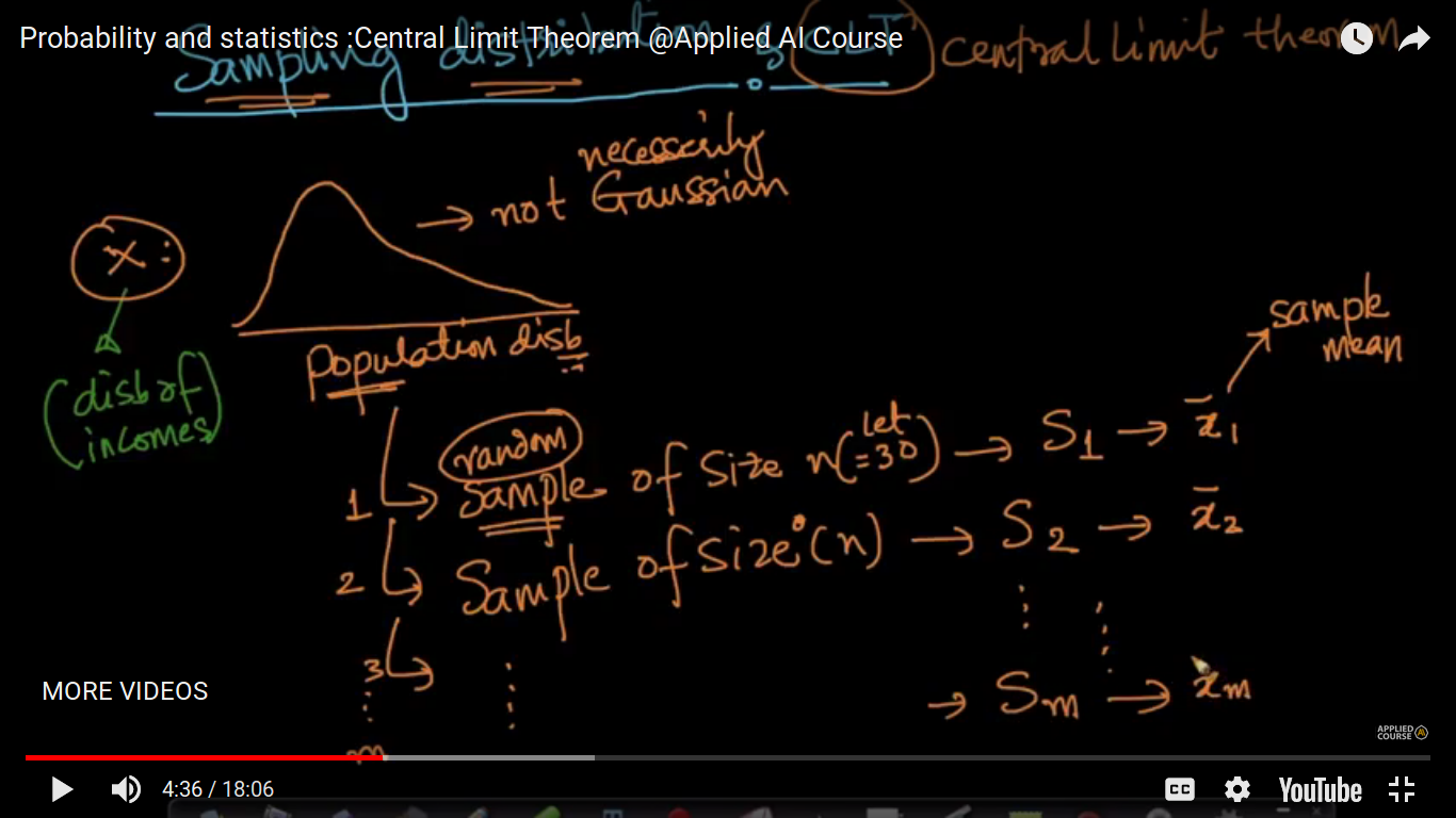
In practice, you do not get to see the all the values of a population. Let us say, you want to estimate the mean height of all humans. It is impossible to have the height of each of the billions of humans in your dataset. What we obtain is a sample of hights of a subset of humans. Now, that is why sample-means are useful and important. Even for a dataset, you do not see the features values for every datapoint int he universe. What you see as a training dataset is only a sample of points.
Please note that we can never get out hands on the population data in most real-world cases as the data may be too large or too hard to obtain. So, CLT helps us estimate the population mean reasonably well, using samples from the population, which are easier to obtain.
No, we are not trying to cross-check the mean. We are trying to estimate the population mean given the sample means. Please note that a “sample” is a subset of observations from the universal_set/population of data-points.
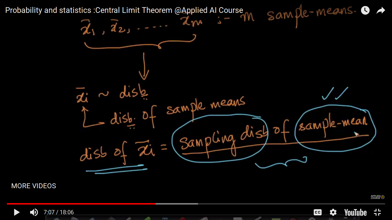
The most important result about sample means is the Central Limit Theorem. Simply stated, this theorem says that for a large enough sample size n, the distribution of the sample mean will approach a normal distribution. This is true for a sample of independent random variables from any population distribution, as long as the population has a finite standard deviation (sigma).
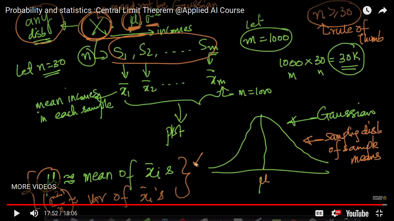
Central Limit Theorem is that the average of your sample means will be the population mean. In other words, add up the means from all of your samples, find the average and that average will be your actual population mean. Similarly, if you find the average of all of the standard deviations in your sample, you’ll find the actual standard deviation for your population
it’s applicable to any general distribution of the random variable.
distribution of the sample means will be approximately normally distributed. This will hold true regardless of whether the source population is normal or skewed
Here, we can easily compute the mean and variance of the distribution, X using PDF.
if n>=30, then any distribution behaves as a normal or Gaussian distribution.
The mean and variance of xi bar become slightly equal to the population Mean and variance/n respectively where n is tending to infinity.
https://stats.stackexchange.com/questions/44211/when-to-use-central-limit-theorem