Description
|
|
Created by Isaac Farias
over 9 years ago
|
|
Page 1
Chapter 20 IPv4 Routing Protocols
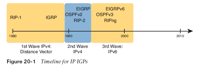
Routers and Layer 3 switches add IP routes to their routing tables using three methods: connected routes, static routes, and routes learned by using dynamic routing protocols.Introduction to Routing ProtocolsEach routing protocol causes routers (and Layer 3 switches) to1. Learn routing information about IP subnets from other neighboring routers2. Advertise routing information about IP subnets to other neighboring routers3. Choose the best route among multiple possible routes to reach one subnet, based on that routing protocol’s concept of a metric4. React and converge to use a new choice of best route for each destination subnet when the network topology changes—for example, when a link failsHistory of Interior Gateway Protocols Historically speaking, RIP Version 1 (RIPv1) was the first popularly used IP routing protocol, with the Cisco-proprietary Interior Gateway Routing Protocol (IGRP) being introduced a little later, as shown in Figure 20-1.
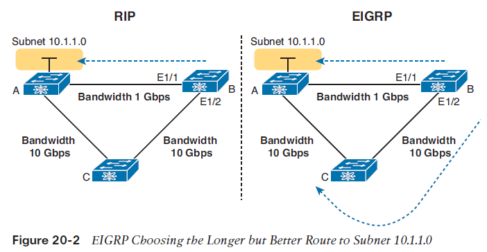
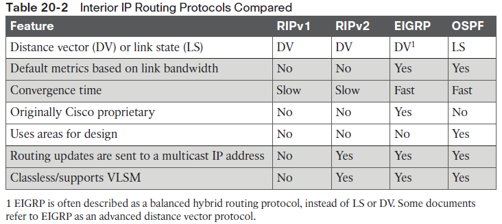
NOTE As an aside, many documents refer to EIGRP’s support for learning IPv4 routes simply as EIGRP, and EIGRP support for IPv6 as EIGRPv6. This book follows that same convention. OSPF RFCs define specific versions, OSPF Version 2 (OSPFv2) learning IPv4 routes, and OSPF Version 3 (OSPFv3) learning IPv6 routes.Comparing IGPsWhat is an IGP in the first place? All the routing protocols mentioned so far in this chapter happen to be categorized as Interior Gateway Protocols (IGPs) rather than as Exterior Gateway Protocols (EGPs). First, the term gateway was used instead of router in the early days of IP routing, so the terms IGP and EGP really do refer to routing protocols. The designers of some routing protocols intended the routing protocol for use inside one companyor organization (IGP), with other routing protocols intended for use between companies and between Internet service providers (ISPs) in the Internet (EGPs).When deploying a new network, the network engineer can choose between a variety of IGPs. Today, most enterprises use EIGRP and OSPFv2. RIPv2 has fallen away as a serious competitor, in part due to its less robust hop-count metric, and in part due to its slower (worse) convergence time.A few key comparison points are as follows:■ The underlying routing protocol algorithm: Specifically, whether the routing protocol used logic referenced as distance vector (DV) or link state (LS).■ The usefulness of the metric: The routing protocol chooses which route is best based on its metric; so the better the metric, the better the choices made by that routing protocol.■ The speed of convergence: How long does it take all the routers to learn about a change in the network and update their IPv4 routing tables? That concept, called convergence time, varies depending on the routing protocol.■ Whether the protocol is a public standard or a vendor-proprietary function: RIP and OSPF happen to be standards, defined by RFCs. EIGRP happens to be defined by Cisco, and until 2013, was kept private.For example, RIP uses a basic metric of hop count. Hop count treats each router as a hop, so the hop count is the number of other routers between a router and some remote subnet. RIP’s hop-count metric means that RIP picks the route with the smallest number of links and routers. However, that shortest route may have the slowest links; a routing protocol that uses a metric based in part on link speed (called bandwidth) might make a better choice. In contrast, EIGRP’s metric calculation uses a math formula that gives routes with slow links a worse metric, and routes with fast links a lower metric, so EIGRP prefers faster routes.As you can see on the left in the figure, RIP on router B chooses the shorter hop route over the top of the network, over the single link, even though that link runs at 1 Gbps. EIGRP, on the right side of the figure, chooses the route that happens to have more links through the network, but both links have a faster bandwidth of 10 Gbps.
On another comparison point, the biggest negative about EIGRP has traditionally been that it required Cisco routers. That is, using EIGRP locked you into using Cisco products, because Cisco kept EIGRP as a Cisco proprietary protocol. In an interesting change, Cisco published EIGRP as an informational RFC in 2013, meaning that now other vendors can choose to implement EIGRP as well. In the past, many companies chose to use OSPF rather than EIGRP to give themselves options for what router vendor to use for future router hardware purchases. In the future, it might be that you can buy some routers from Cisco, some from other vendors, and still run EIGRP on all routers
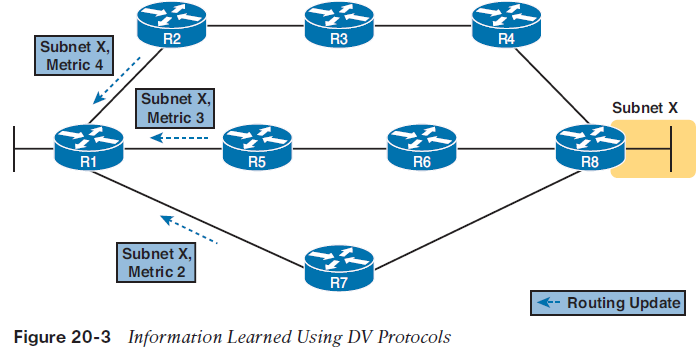
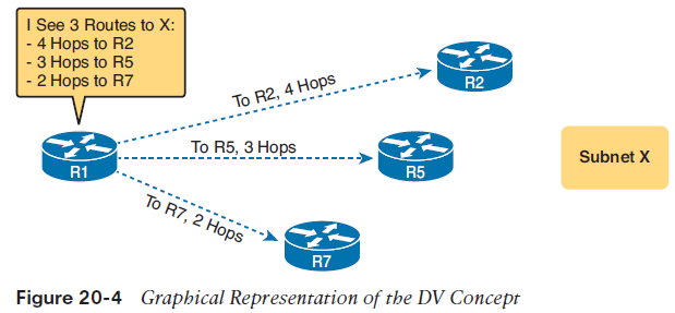
The Concept of a Distance and a Vector The term distance vector describes what a router knows about each route. At the end of the process, when a router learns about a route to a subnet, all the router knows is some measurement of distance (the metric) and the next-hop router and outgoing interface to use for that route (a vector, or direction).The figure shows the flow of RIP messages that cause R1 to learn some IPv4 routes, specifically three routes to reach subnet X:■ The four-hop route through R2■ The three-hop route through R5■ The two-hop route through R7
DV protocols learn two pieces of information about a possible route to reach a subnet:■ The distance (metric)■ The vector (the next-hop router)Figure 20-4 gives a better view into R1’s DV logic. The figure shows R1’s three competing routes to subnet X as vectors, with longer vectors for routes with larger metrics. R1 knows three routes, each with Distance: The metric for a possible route Vector: The direction, based on the next-hop router for a possible route
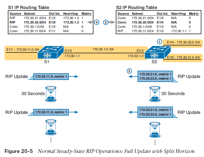
Full Update Messages and Split Horizon Some DV protocols, such as RIP (both RIPv1 and RIPv2), send periodic full routing updates based on a relatively short timer. Specifically, full update means that a router advertises all its routes, using one or more RIP update messages, no matter whether the route has changed or not. So, if a route does not change for months, the router keeps advertising that same route over and over. Figure 20-5 illustrates this concept in an internetwork with two Nexus switches configured as Layer 3 switches, with four total subnets. The figure shows both routers’ full routing tables, and lists the periodic full updates sent by each router. This figure shows a lot of information, so take the time to work through the details. For example, consider what switch S1 learns for subnet 172.30.22.0/24, which is the subnet connected to S2’s E1/4 interface: 1. S2 interface E1/4 has an IP address, and is in an up/up state.2. S2 adds a connected route for 172.30.22.0/24, off interface E1/4, to R2’s routing table.3. S2 advertises its route for 172.30.22.0/24 to S1, with metric 1, meaning that S1’s metric to reach this subnet will be metric 1 (hop count 1). 4. S1 adds a route for subnet 172.30.22.0/24, listing it as a RIP learned route with metric 1.
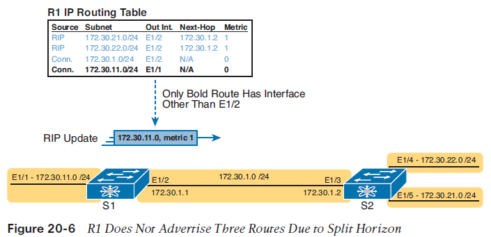
Monitoring Neighbor State with Periodic RIP UpdatesRIPv1 and RIPv2 also send periodic updates, as shown in the bottom of Figure 20-5. That means that each router sends a new update (a full update) on a relatively short time period (30 seconds with RIP).Many of the early DV protocols used this short periodic timer, repeating their full updates, as a way to let each router know whether a neighbor had failed. Routers need to react when a neighboring router fails or if the link between two routers fails. If both routers on a link must send updates every 30 seconds, when a local router no longer receives those updates, it knows that a problem has occurred, and it can react to converge to use alternate routes.Split HorizonFigure 20-5 also shows a common DV feature called split horizon. Note that both routers list all four subnets in their IP routing tables. However, the RIP update messages do not list four subnets. The reason? Split horizon. Split horizon is a DV feature that tells a router to omit some routes from an update sent out an interface. Which routes are omitted from an update sent out interface X? The routes that would like interface X as the outgoing interface. Those routes that are not advertised on an interface usually include the routes learned in routing updates received on that interface. Split horizon is difficult to learn by reading words, and much easier to learn by seeing an example. Figure 20-6 continues the same example as Figure 20-5, but focusing on S1’s RIP update sent out S1’s E1/2 interface to S2. Figure 20-6 shows S1’s routing table with three light-colored routes, all of which list E1/2 as the outgoing interface. When building the RIP update to send out E1/2, split-horizon rules tell S1 to ignore those light-colored routes. Only the bold route, which does not list E1/2 as an outgoing interface, can be included in the RIP update sent out E1/2.
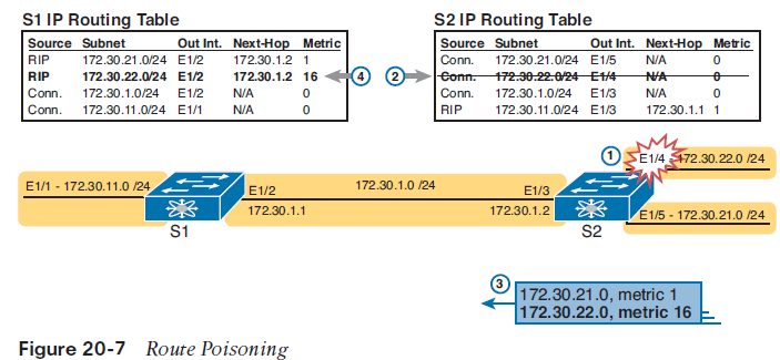
Route Poisoning DV protocols help prevent routing loops by ensuring that every router learns that the route has failed, through every means possible, as quickly as possible. One of these features, route poisoning, helps all routers know for sure that a route has failed. Route poisoning refers to the practice of advertising a failed route, but with a special metric value called infinity. Routers consider routes advertised with an infinite metric to have failed. Figure 20-7 shows an example of route poisoning with RIP, with S2’s E1/4 interface failing, meaning that S2’s route for 172.30.22.0/24 has failed. RIP defines infinity as 16. Figure 20-7 shows the following process: 1. S2’s E1/4 interface fails.2. S2 removes its connected route for 172.30.22.0/24 from its routing table.3. S2 advertises 172.30.22.0 with an infinite metric (which for RIP is 16).4. Depending on other conditions, S1 either immediately removes the route to 172.30.22.0 from its routing table, or marks the route as unusable (with an infinite metric) for a few minutes before removing the route.
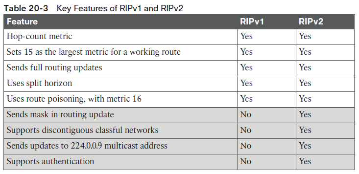
By the end of this process, router S1 knows for sure that its old route for subnet 172.30.22.0/24 has failed, which helps S1 avoid introducing looping IP routes.Each routing protocol has its own definition of an infinite metric. RIP uses 16, as shown in the figure, with 15 being a valid metric for a usable route. EIGRP has long used 2^32 – 1 as infinity (a little more than 4 billion), with some Cisco products bumping that value to 2^56 – 1 (more than 10^16). OSPFv2 uses 2^24 – 1 as infinity.RIP Concepts and OperationThe Routing Information Protocol (RIP) was the first commonly used IGP in the history of TCP/IP. Organizations used RIP inside their networks commonly in the 1980s, and into the 1990s. RIPv2, created in the mid-1990s, improved RIPv2, giving engineers an option for easy migration and co-existence to move from RIPv1 to the better RIPv2Features of Both RIPv1 and RIPv2Like all IGPs, both RIPv1 and RIPv2 perform the same core features. That is, when using either RIPv1 or RIPv2, a router advertises information to help other routers learn routes; a router learns routes by listening to messages from other routers; a router chooses the best route to each subnet by looking at the metric of the competing routes; and the routing protocol converges to use new routes when something changes about the network.RIPv1 and RIPv2 use the same logic to achieve most of those core functions. The similarities include the following:■ Both send regular full periodic routing updates on a 30-second timer, with full meaning that the update messages include all known routes.■ Both use split-horizon rules, as shown in Figure 20-6.■ Both use hop count as the metric.■ Both allow a maximum hop count of 15.■ Both use route poisoning as a loop-prevention mechanism (see Figure 20-7), with hop count 16 used to imply an unusable route with an infinite metric.Differences Between RIPv1 and RIPv2Of course, RIPv2 needed to be better than RIPv1 in some ways, otherwise, what is the point of having a new version of RIP? RIPv2 made many changes to RIPv1: solutions to known problems, improved security, and new features as well. However, while RIPv2 improved RIP beyond RIPv1, it did not compete well with OSPF and EIGRP, particularly due to somewhat slow convergence compared to OSPF and EIGRP.First, RIPv1 had one protocol feature that prevented it from using variable-length subnet masks (VLSMs). To review, VLSM means that inside one classful network (one Class A, B, or C network), that more than one subnet mask is used. For instance, in Figure 20-8, all the subnets are from Class A network 10.0.0.0, but some subnets use a /24 mask, whereas others use a /30 mask.
RIPv1 could not support a network that uses VLSM because RIPv1 did not send mask information in the RIPv1 update message. Basically, RIPv1 routers had to guess what mask applied to each advertised subnet, and a design with VLSM made routers guess wrong.RIPv2 solved that problem by using an improved update message, which includes the subnet mask with each route, removing any need to guess what mask to use, so RIPv2 correctly supports VLSM.RIPv2 changed from using IP broadcasts sent to the 255.255.255.255 broadcast address (as in RIPv1) by instead sending updates to the 224.0.0.9 IPv4 multicast address. Using multicasts means that RIP messages can be more easily ignored by other devices, wasting less CPU on those devices.
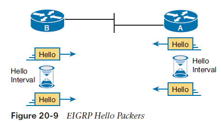
EIGRP Concepts and Operation Enhanced Interior Gateway Routing Protocol (EIGRP) went through a similar creation process as compared to RIP, but with the work happening inside Cisco. Cisco has already created the Interior Gateway Routing Protocol (IGRP) in the 1980s, and the same needs thatdrove people to create RIPv2 and OSPF drove Cisco to improve IGRP as well. Instead of naming the original IGRP Version 1, and the new one IGRP Version 2, Cisco named the new version Enhanced IGRP (EIGRP).EIGRP acts a little like a DV protocol, and a little like no other routing protocol. Frankly, over the years, different Cisco documents and different books (mine included) have characterized EIGRP as either its own category, called a balanced hybrid routing protocol, or as some kind of advanced DV protocol.EIGRP Maintains Neighbor Status Using HelloUnlike RIP, EIGRP does not send full or partial update messages based on a periodic timer. When a router first comes up, it advertises known routing information. Then, over time, as facts change, the router simply reacts, sending partial updates with the new information. The fact that EIGRP does not send routing information on a short periodic timed basis greatly reduces EIGRP overhead traffic, but it also means that EIGRP cannot rely on these updates to monitor the state of neighboring routers. Instead, EIGRP defines the concept of a neighbor relationship, using EIGRP hello messages to monitor that relationship. The EIGRP hello message and protocol defines that each router should send a periodic hello message on each interface, so that all EIGRP routers know that the router is still working.
The routers use their own independent hello interval, which defines the time period between each EIGRP hello. For instance, routers R1 and R2 do not have to send their hellos at the same time. Routers also must receive a hello from a neighbor with a time called the hold interval, with a default setting of three times the hello interval.For instance, imagine both R1 and R2 use default settings of 5 and 15 for their hello and hold intervals. Under normal conditions, R1 receives hellos from R2 every 5 seconds, well within R1’s hold interval (15 seconds) before R1 would consider R2 to have failed. If R2 does fail, R2 no longer sends hello messages. R1 notices that 15 seconds pass without receiving a hello from R2, so then R1 can choose new routes that do not use R2 as a next-hop router to send a frame over the link. Both bandwidth and delay are settings on router interfaces; although routers do have default values for both bandwidth and delay on each interface, the settings can be configured as well.EIGRP calls the calculated metric value the composite metric, with the individual inputs into the formula being the metric components.■ A smaller bandwidth yields a larger composite metric because less bandwidth is worse than more bandwidth.■ A smaller delay yields a smaller composite metric because less delay is better than more delay.EIGRP ConvergenceAnother compelling reason to choose EIGRP as an IGP has to do with EIGRP’s much better convergence time as compared with RIP. EIGRP converges more quickly than RIP in all cases, and in some cases, EIGRP converges much more quickly.With EIGRP, those same worst cases typically experience convergence of less than a minute, often less than 20 seconds, with some cases taking a second or two.EIGRP does loop avoidance completely differently than RIP by keeping some basic topological information. The EIGRP topology database on each router holds some information about the local router, plus some information about the next-hop router in each possible route for each known subnet. That extra topology information lets EIGRP on each router take the following approach for all the possible routes to reach one subnet:■ Similar to how other routing protocols work, a local router calculates the metric for each possible route to reach a subnet, and chooses the best route based on the best metric.■ Unlike other routing protocols, the local router uses that extra topology information to look at the routes that were not chosen as the best route, to find all alternate routes that, if the best route fails, could be immediately used without causing a loop.
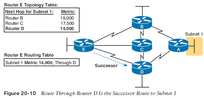
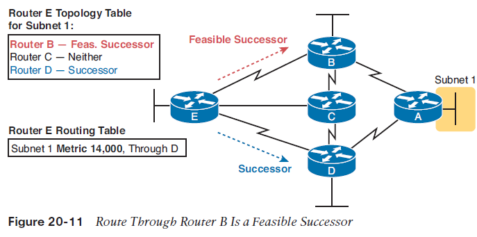
The upper left shows router E’s topology table information about the three competing routes to reach subnet 1: a route through router B, another through router C, and another through router D. The metrics in the upper left show the metrics from router E’s perspective, so router E chooses the route with the smallest metric: the route through next-hop router D. EIGRP on router E places that route, with next-hop router D, into its IP routing table, represented on the lower left of the figure.NOTE EIGRP calls the best route to reach a subnet the successor route.At the same time, EIGRP on router E uses additional topology information to decide whether either of the other routes—the routes through B and C—could be used if the route through router D fails, without causing a loop. Ignoring the details of how router E decides, imagine that router E does that analysis, and decides that E’s route for subnet 1 through router B could be used without causing a loop, but the route through router C could not. Router E would call that route through router B a feasible successor route, as noted in Figure 20-11.
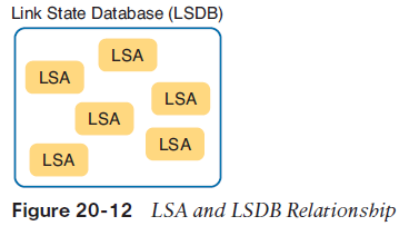
As long as the network stays stable, router E has chosen the best route, and is ready to act, as follows:■ Router E uses the successor route as its only route to subnet 1, as listed in the IPv4 routing table.■ Router E lists the route to subnet 1, through router B, as a feasible successor, as noted in the EIGRP topology table.EIGRP SummaryAs you can see, EIGRP provides many advantages over both RIPv1 and RIPv2. Most significantly, it uses a much better metric, and it converges much more quickly than does RIP.The biggest downside to EIGRP has traditionally been that EIGRP was a Cisco proprietary protocol. That is, to run EIGRP, you had to use Cisco products only. Interestingly, Cisco has published EIGRP as an informational RFC in 2013, so now other vendors could choose to add EIGRP support to their products. Over time, maybe this one negative about EIGRP will fade away.Understanding the OSPF Link-State Routing ProtocolLike EIGRP, OSPF converges quickly. Like EIGRP, OSPF bases its metric by default on link bandwidth, so that OSPF makes a better choice than simplyrelying on the router hop-count metric used by RIP. But OSPF uses much different internal logic, being a link-state routing protocol rather than a distance vector protocol.OSPF Comparisons with EIGRPAlthough EIGRP uses DV logic, and OSPF uses LS logic, OSPF and EIGRP have three major activities that, from a general perspective, appear to be the same:1. Both OSPF and EIGRP use a hello protocol to find neighboring routers, maintain a list of working neighbors, monitor ongoing hello messages to make sure the neighbor is still reachable, and to notice when the path to a neighbor has failed.2. Both OSPF and EIGRP exchange topology data, which each router stores locally in a topology database. The topology database describes facts about the network, but is a different entity than the router’s IPv4 routing table.3. Both OSPF and EIGRP cause each router to process its topology database, from which the router can choose the currently best route (lowest metric route) to reach each subnet, adding those best routes to the IPv4 routing table.For instance, in a network that uses Nexus Layer 3 switches, you could use OSPF or EIGRP. If using OSPF, you could display a Layer 3 switch’s OSPF neighbors (show ip ospf neighbor), the OSPF database (show ip ospf database), and the IPv4 routing table (show ip route). Alternatively, if you instead used EIGRP, you could display the equivalent in EIGRP: EIGRP neighbors (show ip eigrp neighbor), the EIGRP topology database (show ip eigrp topology), and the IPv4 routing table (show ip route). However, if you dig a little deeper, OSPF and EIGRP clearly use different conventions and logic. The protocols, of course, are different, with EIGRP being created inside Cisco and OSPF developed as an RFC. The topology databases differ significantly, with OSPF collecting much more detail about the topology, and with EIGRP collecting just enough to make choices about successor and feasible successor routesBuilding the OSPF LSDB and Creating IP RoutesLink-state protocols build IP routes with a couple of major steps. First, the routers build a detailed database of information about the network and flood that so that all routers have a copy of the same information. (The information is much more detailed than the topology data collected by EIGRP.) That database, called the link-state database (LSDB) , gives each router the equivalent of a roadmap for the network, showing all routers, all router interfaces, all links between routers, and all subnets connected to routers. Second, each router runs a complex mathematical formula (the details of which we can all ignore) to calculate the best route to reach each subnet.Topology Information and LSAs Routers using LS routing protocols need to collectively advertise practically every detail about the internetwork to all the other routers. At the end of the process of flooding the information to all routers, every router in the internetwork has the exact same informationabout the internetwork. Flooding a lot of detailed information to every router sounds like a lot of work, and relative to DV routing protocols, it is. OSPF, the most popular LS IP routing protocol, organizes topology information using linkstate advertisements (LSAs) and the link-state database (LSDB). Figure 20-12 represents the ideas. Each LSA is a data structure with some specific information about the network topology— for instance, each router must be described by a separate LSA. The LSDB holds the collection of all the LSAs known to a router. Think of the LSDB as having one LSA for every router, one for every link, with several other types as well.
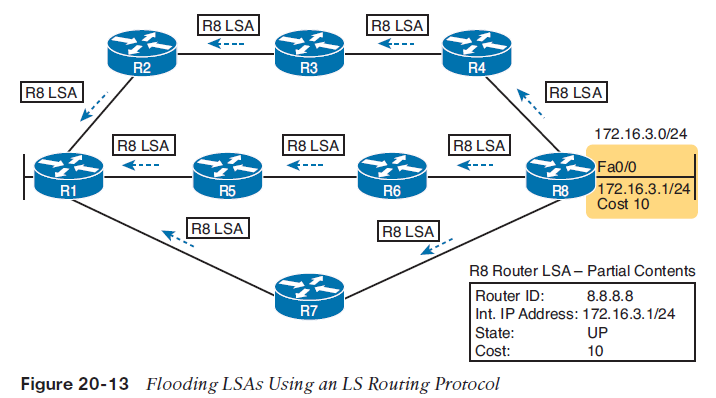
LS protocols rely on having all routers knowing the same view of the network topology and link status (link state) by all having a copy of the LSDB. The idea is like giving all routers a copy of the same updated road map. If all routers have the exact same road map, and they base their choices of best routes on that same road map, then the routers, using the same algorithm, will never create any routing loops. To create the LSDB, each router will create some of the LSAs needed. Each router floods both the LSAs it creates, plus others learned from neighboring routers, so that all the routers have a copy of each LSA. Figure 20-13 shows the general idea of the flooding process, with R8 creating and flooding an LSA that describes itself (called a router LSA). The router LSA for router R8 describes the router itself, including the existence of subnet 172.16.3.0/24, as shown on the right side of the figure. (Note that Figure 20-13 actually shows only a subset of the information in R8’s router LSA.)
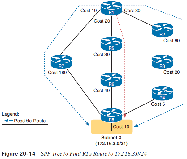
Figure 20-13 shows the rather basic flooding process, with R8 sending the original LSA for itself and with the other routers flooding the LSA by forwarding it until every router has a copy. The flooding process has a way to prevent loops so that the LSAs do not get flooded around in circles. Basically, before sending an LSA to yet another neighbor, routers communicate and ask “do you already have this LSA?” Then they avoid flooding the LSA to neighbors that already have it.Applying Dijkstra SPF Math and OSPF Metrics to Find the Best RoutesAll LS protocols use a type of math algorithm called the Dijkstra shortest path first (SPF) algorithm to process the LSDB. That algorithm analyzes (with math) the LSDB, and builds the routes that the local router should add to the IP routing table—routes that list a subnet number and mask, an outgoing interface, and a next-hop router IP address.The sum of the OSPF interface costs for all outgoing interfaces in the routeThe OSPF metric for a route is the sum of the interface costs for all outgoing interfaces in the route. By default, a router’s OSPF interface cost is actually derived from the interface bandwidth: The faster the bandwidth, the lower the cost. So, a lower OSPF cost means that the interface is better than an interface with a higher OSPF cost.Armed with the facts in the previous few paragraphs, you can look at the example in Figure 20-14 and predict how the OSPF SPF algorithm will analyze the available routes and choose a best route. This figure features the logic on router R1, with its three competing routes to subnet X (172.16.3.0/24) at the bottom of the figure.
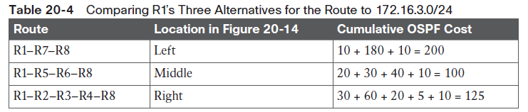
NOTE OSPF considers the costs of the outgoing interfaces (only) in each route. It does not add the cost for incoming interfaces in the route.Table 20-4 lists the three routes shown in Figure 20-14, with their cumulative costs, showing that R1’s best route to 172.16.3.0/24 starts by going through R5.
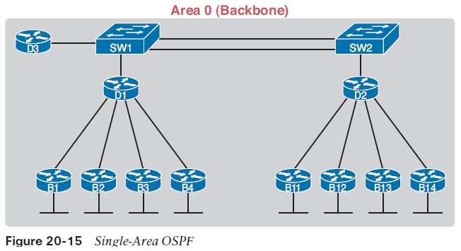
As a result of the SPF algorithm’s analysis of the LSDB, R1 adds a route to subnet 172.16.3.0/24 to its routing table, with the next-hop router of R5.NOTE OSPF calculates costs using different processes depending on the area design.The example surrounding Figure 20-14 best matches OSPF’s logic when using a single area design.Scaling OSPF Through Hierarchical DesignOSPF can be used in some networks with very little thought about design issues. You just turn on OSPF in all the routers, and it works! However, in large networks, engineers need to think about and plan how to use several OSPF features that allow OSPF to scale well. For instance, the OSPF design in Figure 20-15 uses a single OSPF area, because this small internetwork does not need the scalability benefits of OSPF areas.Using a single OSPF area for smaller internetworks, as in Figure 20-15, works well. The configuration is simple, and some of the hidden details in how OSPF works remain simple. In fact, with a small OSPF internetwork, you can just enable OSPF, with all interfaces in the same area, and mostly ignore the idea of an OSPF area.
Now imagine a network with 900 routers, instead of only 11, and several thousand subnets. In that size of network, the sheer amount of processing required to run the complex SPF algorithm might cause convergence time to be slow just because of the time it takes each router to process all the math. Also, the routers might experience memory shortages. The problems can be summarized as follows: ■ A larger topology database requires more memory on each router.■ The router CPU time required to run the SPF algorithm grows exponentially with the size of the LSDB.■ With a single area, a single interface status change (up to down, or down to up) forces every router to run SPF again! OSPF provides a way to manage the size of the LSDB by breaking up a larger network into smaller pieces using a concept called OSPF areas.OSPF then creates a separate and smaller LSDB per area, rather than one huge LSDB for all links and routers in the internetwork. With smaller topology databases, routers consume less memory and take less processing time to run SPF. OSPF multi-area design puts all ends of a link—a serial link, and VLAN, and so on—inside an area. To make that work, some routers (Area Border Routers, or ABRs) sit at the border between multiple areas. Routers D1 and D2 serve as ABRs in the area design shown in Figure 20-16, which shows the same network as Figure 20-15, but with three OSPF areas (0, 1, and 2).Figure 20-16 shows a sample area design and some terminology related to areas, but it does not show the power and benefit of the areas. By using areas, the OSPF SPF algorithm ignores the details of the topology in the other areas. For example, OSPF on router B1 (area 1), when doing the complex SPF math processing, ignores the topology information about area 0 and area 2. Each router has much less SPF work to do, so each router more quickly finishes its SPF work, finding the currently best OSPF routes.
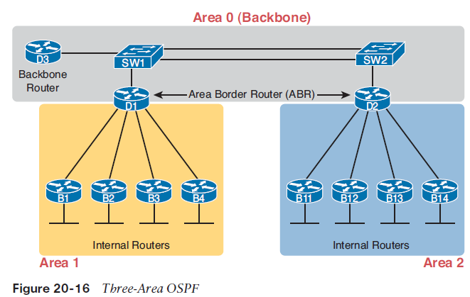
Page 2
Want to create your own Notes for free with GoConqr? Learn more.