
Karteikarten
Stats S1
Karten in diesem Stapel (60)
- 1PopulationRefers to the entire set of data that exists
- 2SampleA representative part of the population
- 3Sampling frameAssigns a number to every member of the population
- 4Random sampleGives every member of the population an equal chance of being chosen
- 5Relative frequency\(Relative frequency=\frac{frequency}{total frequency}\)
- 6Histogramsrepresent continuous data; height of columns determined by freq. density; area of columns gives you the freq.; no gaps between the upper and lower class boundaries
- 7UCB and LCB (upper and lower class boundaries)lcb = 50g and ucb = 250g may be expressed as
"100-200 to nearest 100g"
"\(50\leq mass <250g\)"
"50-" followed by "250-" for the next class - 8Frequency polygonsjoin the MIDPOINTS of each interval together with STRAIGHT LINES;
at each end of the polygon we plot the midpoint of where the previous/next interval would be - 9Frequency curveFor if we want to infer general shape of population distribution (instead of sample data distribution as with a frequency polygon)
- 10Cumulative frequency polygonjoined with straight lines;
plotted at the ENDS of the intervals - 11Box and whisker plotsConvenient way of representing range, quartiles and IQR
For discrete or continuous data - 12Mean \(\bar{x}\)\(\frac{\Sigma x}{n}\) or \(\frac{\Sigma fx}{\Sigma f}\)
- 13MedianMiddle value when ordered \(\frac{n+1}{2}\)th value
If this isn't a whole number, take the average of the terms either side - 14Estimating mean (for grouped data)Estimate the mean by using midpoints (\(\frac{ucb+lcb}{2}\))
- 15Estimating the median (for grouped data)Use linear interpolation (assume all values are evenly spread)
- 16Usefulness of the Mean+good average because you use ALL your data to calculate
- heavily affected by extreme values/outliers
- can only be used with qualitative data - 17Usefulness of Median+ less affected by extreme values/outliers
+ provides info about the spread of values
- only uses part of the data - 18Usefulness of Mode+can be used with qualitative data
- some data sets can have more than one mode (and if every value in a data set occurs just once, then mode isn't helpful) - 19coding and scalingsubtracting (coding) or dividing (scaling) to make the mean easier to calculate
- 20Finding the mean using coding and scalingIf \(y=\frac{x-b}{a}\) then \(\bar{y}=\frac{\bar{x}-b}{a}\)
- 21Finding the standard deviation using coding and scalingIf \(y=\frac{x-b}{a}\) then \(S_y=\frac{S_x}{a}\)
Standard deviation is only changed by multiplying or dividing. If you used coding, the standard deviation would be unchanged. - 22Quartiles\(Q_1=\frac{n}{4}\) and \(Q_3=\frac{3n}{4}\)
If you get an integer, find the average of this term and the one above
If you get a decimal, round the number up to find the position - 23PercentilesDivide the data into 100
E.g. \(11^{th}\) percentile \((P_{11})\) is \(\frac{11}{100}\) x total frequency - 24Inter-percentile rangeSubtract two percentiles
E.g. the middle 60% of readings = \(P_{80}-P_{20}\) - 25Variance \(s^2\), and standard deviation s, \(\sigma\)\(s^2=\frac{\Sigma x^2}{n}-\bar{x}^2\) or \(s^2=\frac{\Sigma fx^2}{\Sigma f}-\bar{x}^2\)
"The mean of the squares minus the square of the mean" - 26Outliers- make standard deviation and variance much larger than they should be
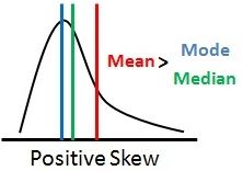
- if a data set contains outliers then a better measure of dispersion is the IQR - 27Positive SkewTail on the right, a lot of readings on the low side
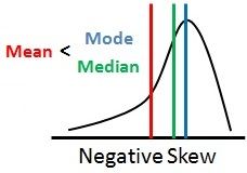
- 28Negative SkewTail on the left, a lot of readings on the high side
- 29Coefficient of skewnessMeasures how "all-up-one-end" the data is and is usually between -3 and 3
- 30Pearson's coefficient of skewness\(=\frac{mean - mode}{standard deviation}\)
- 31Quartile coefficient of skewness\(=\frac{(Q_3 - Q_2)-(Q_2-Q_1)}{Q_3-Q_1}\)
Difference between UQ and Median, minus the difference between the LQ and the median, divided by IQR - 32Comparing distributions: LOCATIONwhich has the higher mean, median, quartiles? These show which distribution has generally higher values.
- 33Comparing distributions: DISPERSIONLook at IQR, range, standard deviation. Higher values show that the data is more varied/spread out.
- 34Comparing distributions: SKEWNESSNegative skew- lower values are more spread out/higher values more tightly bunched
Positive skew- higher values are more spread out/lower values more tightly bunched - 35Venn diagramsstart with the values in the middle and work your way out
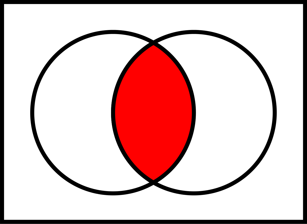
- 36Intersection of A and B: \(P(A\cap B)\)
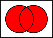
- 37Union of A and B: \(P(A\cup B)\)\(P(A\cup B)=P(A)+P(B)-P(A\cap B)\) *in F.B.*
- 38—\(P(A`)=1-P(A)\)
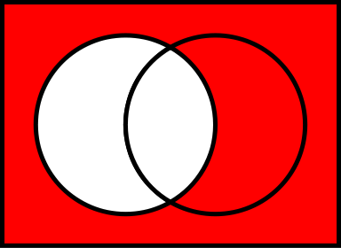
- 39Mutually exclusive eventscan't happen at the same time
i.e.\(P(A\cap B)=0\) and \(P(A\cup B)=P(A)+P(B) - 40\(P(A\mid B)\)means "probability of A, given that B has happened"
- 41\(P(B\mid A`)\)
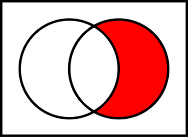
- 42Conditional Probability\(P(a\mid B)=\frac{P(A\cap B)}{P(B)}\) and rearranging: \(P(A\cap B)=P(B)P(A\mid B)\) *in F.B.*
- 43Independent EventsUse these to test if events are independent \(P(A\mid B)=P(A)\) or \(P(B\mid A)=P(B)\) and \(P(A\cap B)=P(A)P(B)\)
- 44Permutations of distinguishable objectsn is number of objects and r is number of spaces: \({}^nP_r = \frac{n!}{(n-r)!}\)
E.g. arranging 5 different objects in groups of 3 becomes \({}^5P_3=\frac{5!}{2!}\) - 45Permutations of indistinguishable objectsn is number of objects and r is number of indistinguishable objects: \({}^nP_{n-r} = \frac{n!}{r!}\)
E.g. arrangments of the letters JOMOSS (2 Os and 2 Ss) \(=\frac{6!}{2!2!}\) - 46CombinationsOrder is not important
Choosing r things out of n distinguishable things \({}^nC_r=\frac{n!}{(n-r)!r!}\) or \(\binom{n}{r}\)
E.g. Choosing 3 out of my 5 favourite books: \({}^5C_3=\frac{5!}{2!3!}=10\) - 47Discrete Random Variable XThe probabilities of all possible values of X add up to 1
- 48Cumulative distribution function F(x)A running total of probabilities. Gives the probability that X will less than or equal to a particular value.
- 49If X is a discrete random variable and 'a' is a constant E(a)=.... E(aX+b)=....E(a) = a
E(aX+b) = aE(X) + b - 50If X is a discrete random variable and 'a' is a constant E(aX+bY)=....E(aX+bY) = aE(X) + bE(Y)
- 51If \(f_1(X)\) and \(f_2(X)\) are any two functions of X \(E(f_1(X) + f_2(X) =\)\(E(f_1(X) + f_2(X)) = E(f_1(X)) + E(f_2(X))\)
- 52If X is a discrete random variable and 'a' and 'b' are constants Var(a)= Var(aX)= Var(aX+b)=\(Var(a)=0\)
\(Var(aX)=a^2Var(X)\)
\(Var(aX+b)=a^2Var(X)\) - 53Discrete uniform distributionThe probabilities are equal for every value of X
- 54Mean and variance for a discrete uniform distribution X with consecutive whole number values a, a+1, a+2,..., b\(E(X)=\frac{a+b}{2}\)
\(Var(X)=\frac{(b-a+1)^2-1}{12}\) - 55PMCC Product moment correlation coefficientMeasures how close to a straight line the points on a scattergraph lie.
perfect positive: \(r=+1\)
perfect negative: \(r=-1\)
no correlation: \(r=0\) - 56Drawing a regression lineAlways goes through \((\bar x\,\bar y)\)
Estimate one other coordinate set (using formula for regression line). Circle both points and join them. - 57Residual from linear regressionResidual = observed value - estimated value
Mark on graph with a line from point to regression line - 58Estimating values using regression lineEstimates are unreliable if extrapolating beyond the range of x for which we have data
- 59Normal Distributiontransform to z using \(\frac{x-\mu}{\sigma}\) and look up in z tables
- 60Percentage points table\(P(Z>z)=0.05\) using tables \(z=1.6449\)
\(P(Z
Informationen
- Beschreibung
- A level Maths Karteikarten am Stats S1, erstellt von Joanne Moss am 04/05/2017.
- Erstellt von
- Joanne Moss
- Aufrufe
- 1
- Bewertung