Linear regression

Linear regression

1. summary(mod) gives inf about call, residuals, coefficients = slope + intercept, R^2, RMSE = residual SE

2. residuals(mod) gives inf about .hat = leverage and .cooksd = influence

3. Coefficient of determination R^2 can be computed as 1-(SSE/SST) = 1-(Var(e)/Var(y)), e=vector of residuals, y=response. Therefore R^2=percentage of variability in response that is explained by the model, since residuals are part of that variability remaining unexplained by the model.

   • # Compute SSE for regression model mod_hgt: mod_hgt %>% summarize(SSE = var(.resid)). SSE is computed by using SUMMARIZE function on AUGMENTed data: mod %>% augment() %>% summarize(SSE = sum(.resid^2), SSE_also = (var(.resid)*(n()-1))
     • R^2 gives us measurement of the strength of fit relative to null model, in which all fitted values = mean(y) and since SSE = SST the R^2 for null model = 0
       • Compute RMSE (=the root mean squared error, a.k.a. residual standard error.) by adding up squared residuals of the model and dividing this sum by the number of degrees of freedom sqrt(sum(residuals(mod)^2) / df.residual(mod)) [1] 9.30804 RMSE=SSE/n-2, where n-2 are degrees of freedom
         • by using summary(mod) you'll get residual standard error: 9.308 on 505 degrees of freedom
         • One way to assess strength of fit is to consider how far off the model is for a typical case. For some observations, fitted value Y^will be very close to actual Y, while for others it will not. The magnitude of a typical residual gives us a sense of how close our estimates are.
         • Some of residuals are positive, while others are negative (below regr. line). Least squared fitting procedure guarantees that the mean of residuals = 0. Therefore, it makes sense to compute square root of the mean of errors = RMSE
     • SST stands for total sum of the squares - this is a measure of the variability in the response variable. By building a regression model, we hope to explain some of that variability. The portion of SST that is not explained by the model is SSE.
       • For least squared regression models with a single explanatory variable the value of R2 is just the square of the correlation coefficient.

4. The leverage of an observation in a regression model = distance of that observation from the mean of the explanatory variable. That is, observations close to the mean of X have low leverage, while observations far from the mean of the explanatory variable have high leverage. Points of high leverage may or may not be influential. The augment() function from the broom package will add the leverage scores (.hat) to a model data frame.

   • Influence depends on leverage (taking only X into account) and magnitude of residuals (depending on response Y and fitted values Y^)
     • We measure influence using Cook's distance, which incorporates both the leverage and residual of each observation.
       • Leverage and influence help us understand how outliers affect out regression model
         • # Rank influential points: library(broom) mod %>% augment() %>% arrange(desc(.cooksd)) %>% head()

5. nontrivial_players <- mlbBat10 %>% filter(AB >= 10 & OBP < 0.500)

   • mod_cleaner <- lm(SLG ~ OBP, nontrivial_players)
     • # Visualize new model: ggplot(nontrivial_players, aes(x = OBP, y = SLG)) + geom_point() + geom_smooth(method = "lm")
       • by removing outliers and re-fitting the model, better model fit can be achieved. One must have strong justification for it! Here outlier with OBP = 0.55 was a valid data point. Predictions of the model are now skewed.

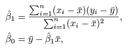
6. model coefficients = Intercept beta zero and Slope= beta one. Y ≈ β0 + β1X.

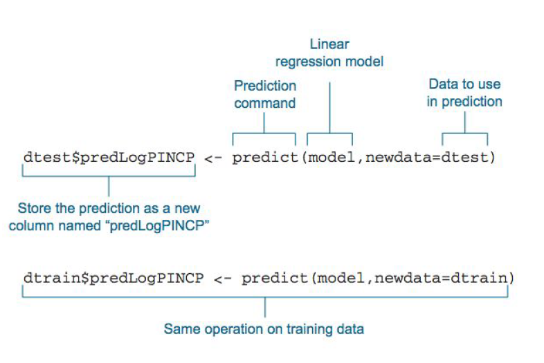
   • we can predict future sales on the basis of a particular value of TV advertising by computing ˆy = ˆ β0 + ˆ β1x, where ˆy indicates a prediction of Y on the basis of X = x.
     • Our goal is to minimize the vertical distance between all the data points and our line and to obtain coefficient estimates ˆ β0 and ˆ β1 such that the linear model fits the data well so that the line is close to data points. There are lots of different ways to minimize this, (sum of squared errors, sum of absolute errors, etc), but all these methods have a general goal of minimizing this distance ex. minimizing the least squares.
       • Standard errors can be used to compute confidence intervals. A 95% confidence is defined as a range of values such that with 95% interval probability, the range will contain the true unknown value of the parameter.
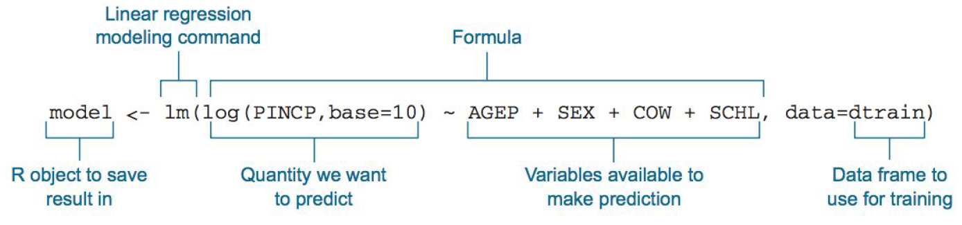
     • The general model of building a linear regression model in R looks like this: model <- lm(y ~ x1 + x2,data) or to use all the features in your data: model <- lm(y ~. , data) # Uses all features

7. summary(mod)

   • Residuals are the difference between the actual values of the variable you're predicting and predicted values from your regression--y - ŷ.
     • If the residuals are normally distributed, the mean of the difference between our predictions and the actual values is close to 0 (good) = like a dartboard. When the model doesn't hit the bullseye, it's missing in all of the other buckets evenly but still close to the bullseye as opposed to on the outer edges of the dartboard.
   • t-value of the coefficient estimates: score that measures whether or not the coefficient for this variable is meaningful for the model. T-value is used to calculate the p-value and the significance levels.
     • p-value: probability that the variable is NOT relevant. You want this number to be as small as possible. If the number is really small, R will display it in scientific notation.
       • Significance stars are shorthand for significance levels, with the number of asterisks displayed according to the p-value computed. *** for high significance and * for low significance.
         • In this case, *** indicates that it's unlikely that no relationship exists ex. b/w absences and G3 scores => this means without double negatives: relationship b/w those 2 variables is very likely
   • Estimate: the estimated coefficient is the value of slope calculated by the regression.
   • Std. Error: measure of the variability in the estimate. Lower means better but this number is relative to the value of the coefficient. As a rule of thumb, you'd like this value to be at least an order of magnitude less than the coefficient estimate.
   • Significance codes: The more punctuation there is next to your variables, the better. Blank=bad, Dots=pretty good, Stars=good, More Stars=very good
   • The Residual Std Error is just the standard deviation of residuals. You'd like this number to be proportional to the quantiles of the residuals. For a normal distribution, the 1st and 3rd quartiles should be 1.5 +/- the std error.
     • The Degrees of Freedom is the difference b/w the number of observations included in your training sample and the number of variables used in your model (intercept counts as a variable).
   • R-squared: metric for evaluating the fit of your model. Higher is better with 1 being the best. Corresponds with the amount of variability in what you're predicting that is explained by the model. WARNING: While a high R-squared indicates good correlation, correlation does not always imply causation.
   • F-statistic & resulting p-value: R performs an F-test on the model. This takes the parameters of our model (1) and compares it to a model that has fewer parameters (2). In theory the model with more parameters (1) should fit better. If (1) doesn't perform better than (2), the F-test will have a high p-value (probability NOT significant boost). If (1) is better than (2), you will have a lower p-value. The DF, or degrees of freedom, pertains to how many variables are in the model. In our case there is one variable so there is one degree of freedom.

Bilder und Dateien der Mindmap