3003PSY Stats Notes

Página 1

Week 1

CHARACTERISTICS OF GOOD PSYCHOLOGICAL RESEARCH

Guided by theory

Standardised procedures

Generalisable- internal and external validity

Reliable

Uses multiple methods including experimental, correlational and descriptive research

The twin tools of science

Research methodology

The collection of approaches, paradigms and procedures (real or logical) that give us confidence in whatever data we gather

Statistical analysis

Algorithms with which we process our (usually quantitative) data to help us to arrive at a conclusion… • … about our research question

Name your assumptions

We believe that our constructed world is a system of integrated causes and effects

We believe that carefully planned and executed empirical research can help us ultimately to uncover these - not everyone thinks so

We believe that it is feasible to assign numbers (in most cases) to measure these

We are willing to make certain assumptions about the numbers (representing the causes and effects) and their relationships.

Statistical procedures are a limited set of mathematicallyderived tools used in modelling research questions, taking our numbers as input

Statistics are decision aids

Doing research

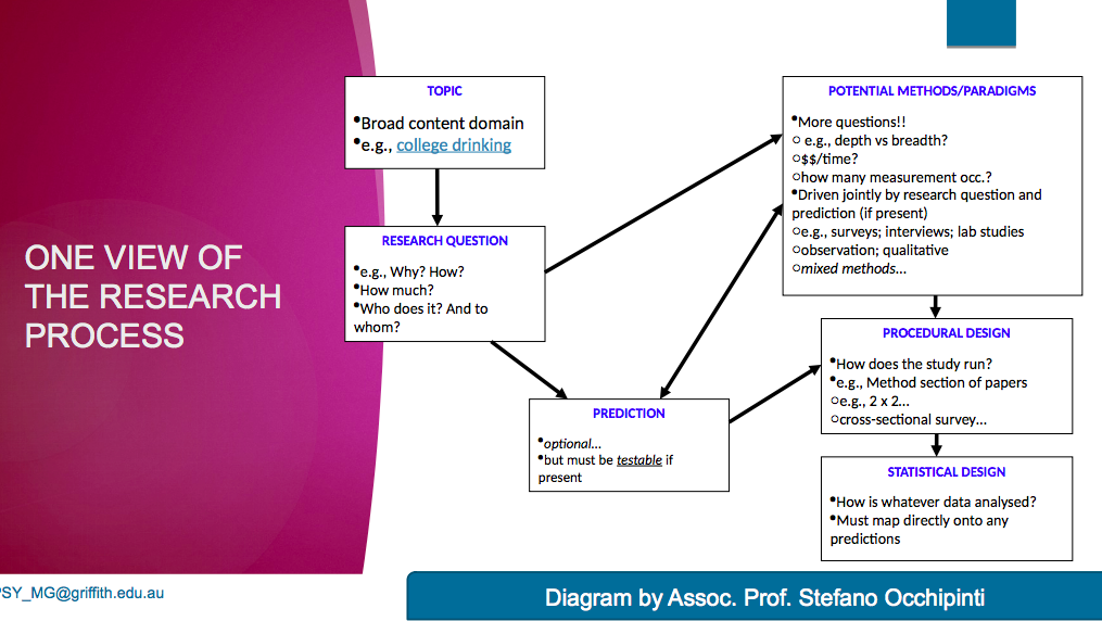
Researchers begin with a question usually derived from a topic area of particular interest

The research question guides and shapes the rest of the process It may push us to choose a particular set of methods

E.g., a survey vs an experiment; a probability sample vs a convenience sample

The statistics will follow from this as well

Research Question

Basic question researcher wants to answer

Often, there is more than one research question.

Precedes any predictions

Think in terms like:

How? How much? Who? Why?

How does drinking change across first year?

What are the correlates of college drinking?

What are the predictors of college drinking?

Each of these suggests different approaches to sampling, study design and analysis…

Predictions:

These must be testable

Some state of the world that data will address

Our models of science based on falsification  Hypotheses should be falsifiable It is not always the case that we make a prediction…  …but often, we have enough empirical data and theory to guide us and so we do make one  You can’t just opt out of your own accord…

Design

Really, it splits up into the procedural part this is probably what you thought of as “The design”

E.g., 2 x 2 experimental study

A mailout survey (or an online survey)

The statistical part

Many statistics that you have learned are tied intimately to a design but not always so Important to understand this as we ask more complex, real-world (!) questions

Página 2

Week 2

Questions:

1. Research question

What is the research question and what type of question is it?

What is the significance of the research question?

2. A prediction

What is/are the prediction(s) of the study (where appropriate)?

3. A way (design and/or procedure) to test it

Will the design be experimental or correlational, or a mixture?

true- or quasi- experimental, correlational?

Cross-sectional or longitudinal?

How will each variable be manipulated/measured?

Most importantly, is the type of design/procedure appropriate to the Research Question— are there any other approaches or paradigms that might work as well, or better?

Are there likely to be hidden issues, such as retrospective data etc.?

Outline the procedures you would employ

How will each variable be manipulated/measured?

Are there any constraints imposed by the social or political/ethical context?

Is it clear how the intended design will provide data to test the prediction?

How long would it take to run the study?

CONSTRUCTS, VARIABLES, & MEASUREMENT

Surveys are a particular form of non-experimental data gathering

As almost all of the key variables in survey approaches are measured and not manipulated experimentally, we need to spend a lot more time focusing on how to get reliable and valid measures

Considering best ways to tap constructs

Many different ways: behaviours, peer or self reports etc

CONSTRUCTS-VARIABLES-OPERATIONS

Attitudes Toward Statistics - is an abstract concept

We construct construct the idea of the thing—does not exist by itself the idea of the thing—does not exist by itself

not directly observable - construct

e.g., attitude, parenting skill, anxiety, personality traits

We use measures we believe will tap the constructs

e.g., self-report measures, Explicit attitude scale; psychophysiological measures etc

These are our variables

We create scores from the measures create scores from the measures

e.g., total score on a perfectionism scale, the averaged output of psychophysiology

measures are all operations or operational definitions

operation = where do the actual numbers (in SPSS) come from?

Goodness of measures:

Need to be able to trust our measurements, or our results can be brushed aside immediately

This involves matters of degree and it is formalised as reliability and validity

it’s not a black and white judgement

reliability based on random error

validity based on coverage of correct underlying construct

All we have are the observed scores…

COMPONENTS OF OBSERVED SCORES

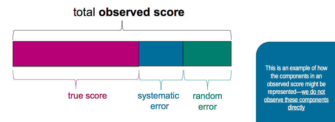
Any time a measurement is made it is influenced by a range of factors—it represents 3 things

The systematic effect of the underlying construct [true score]

e.g., how much I actually know stats

E.g., should be unchanging across occasions without some treatment to increase (or decrease) it

Unrelated but systematic factors [systematic error]

e.g., how well I perform in testing situations in general

People with low test anxiety systematically better than high test anxiety people

Chance, changeable factors [random error]

Whether or not I happened to get little sleep one night at random

Measurement

The reliability and validity of survey measures is the basis on which all of this rests and must be uppermost in our minds as we design measures and variables.

All we have to start with is well chosen and operationalised measures!

In particular, the more systematic and random error there is in our measures, the harder it is to make any sort of inference

We need to maximise (or better, optimise) the amount of true score in our measures

Reliabilty and Validity

Reliability:

Test-retest reliability - the stability of the measurement across time

Determined by administering the same measure on two occasions and looking at the correlation between the scores.

The more stable the measure, the stronger the correlation.

The time frame between testing can vary from several days to several years, depending on the construct being measured.

For instance, scores on an intelligence test taken in adulthood should remain stable over the years, whereas scores on a reading or vocabulary test will change rapidly during early childhood.

Internal consistency - the extent to which items on a measure assess the same construct

A measure needs to be internally consistent.

Items measuring a construct should correlate strongly with each other.

There are a number of ways to assess internal consistency.

One frequently used method is referred to as split-half reliability.

An instrument is administered and divided into halves that are scored separately. One half of the test can then be correlated with the other.

An alternative method used for determining an instrument’s internal consistency is the use of a statistic known as Cronbach's alpha, which is based on the average correlation of all the possible split-halves within a test.

The recommended minimal criterion for an alpha coefficient is .7.

Inter-rater reliability - the level of agreement between two or more raters

Inter-rater reliability is relevant to assessments in which two or more trained observers arrive at some conclusion, such as diagnosis.

Although there are a variety of coefficients assessing inter-rater reliability, the most commonly used coefficient is the Kappa statistic, which measures the level of agreement between two or more observers on categorical outcomes (e.g., illness/no illness).

Kappas range from 0-1, with coefficients closer to 1 indicating that two observers agree more often than chance. Generally a Kappa of .70 or greater is considered acceptable.

Intra-class correlations (ICC) are also frequently used for agreement on measures that derive a score rather than a categorical decision.

Validity:

Content Validity

An measure is considered to have content validity if it measures all aspects of the construct of interest.

Construct Validity

Construct validity requires that the measure assesses only those characteristics of the construct it was designed to measure.

Two related forms of construct validity are convergent and discriminant validity.

Convergent validity is established when the measure correlates highly with other tests or methods of measuring the same construct.

For example, a self-report measure of depression should correlate highly with a clinician’s assessment of depression or with another established measure of depression

Discriminant validity is established in the presence of low correlations between the measure and measures of other unrelated constructs.

For example the above measure of depression should not correlate with a measure of intelligence.

Criterion Validity

Criterion validity refers to the extent to which it corresponds to another accurate measure of the construct. This can be tested at a single point in time - concurrent validity or as a predictor of future outcomes - predictive validity.

Concurrent validity refers to the relationship between scores on the measure of interest and another measure of the same construct or a diagnosis at the same time.

For example a measure a depression severity should be associated with other standardised measures of depression or a major diagnostic system such as the DSM-IV.

Predictive validity is the extent to which an individual’s scores on a measure will accurately predict that individual’s future scores or behaviour.

For instance, a measure of hazardous alcohol use, in which high scores in adolescence consistently predict alcohol use problems in adulthood, would be considered to have predictive validity.

SAMPLING BIAS AND SAMPLING ERROR

Inferential Statistics - using sample data to make inferences about population parameters - if nothing else is known, the statistics of a sample (e.g., the mean) are the best estimates of the population parameters (e.g., height of Griffith students based on this class).

But samples may fail to provide good estimates of population for two reasons: (1) sampling bias and (2) sampling error

Sampling Bias:

Due to faulty sampling methods, some important subgroups of the population may be over- or under-represented in our sample

Systematic variation

A classic example…

American election in the 1948 Polls predicted the Republican candidate, Thomas Dewey would win

However, the Democrat, Harry S. Truman, won by a landslide

Avoidable through random sampling: Ideally, every member of target population should be equally likely to be selected for the sample

Sampling error:

the term ‘sampling error’ implies a mistake but this is misleading … it’s a natural thing and can’t be helped.

Think of this as sampling fluctuation

so the question is not whether the sample mean differs from the population mean (it almost always will) but how likely is it that the difference we observed could have occurred by chance

Sampling Distribution

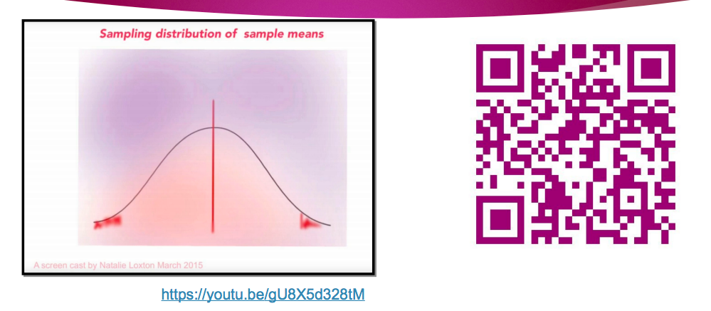
The distribution of a statistic that we would expect if we drew an infinite number of samples (of a given size) from the population

Sampling distributions have means and SDs

Can have a sampling distribution for any statistic, but the most common is the sampling distribution of the mean

In a future week we will discuss the sampling distribution of the correlation coefficient

Standard error of mean

standard error of the mean is the standard deviation of the distribution of sample means

it represents the typical or average distance between a sample mean and the mean of the population

it is used to define and accurately measure sampling error

Sampling distribution:

Página 3

Week 3

What is a survey:

Survey = set of questions tapping one or more constructs that are administered to a sample of participants. This is a survey study!

Unlike a lab study in which sampling considerations are given less weight, a survey study is heavily dependent on the sampling for validity—future weeks

a survey instrument tends to contain all measured variables, either continuous scales or attributes (nominal, ordinal)

Can be administered once (cross-sectional) or more than once to the same people (panel or longitudinal, if linked)

also various combinations and cohort designs

Can be interviews

Can be written

Self-report measures

Conducting a survey study:

What is/are my research question(s)??

What is my budget in $$ and time?

Cost is a big driver in research data gathering

Online = cheapest, Face to Face = most expensive

Cost is correlated fairly well with response rate, sample quality and Participants’motivation

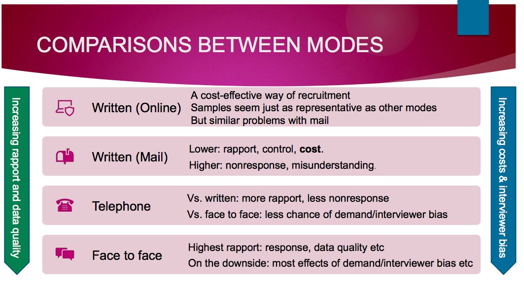
Comparison between modes:

Written (Online)

A cost-effective way of recruitment

Samples seem just as representative as other modes

But similar problems with mail

Written (Mail)

Lower: rapport, control, cost.

Higher: nonresponse, misunderstanding

Telephone

Vs. written: more rapport, less nonresponse

Vs. face to face: less chance of demand/interviewer bias

Face to face

Highest rapport: response, data quality etc

On the downside: most effects of demand/interviewer bias etc

Potential problems with survey data:

Misunderstanding the question

Ps not having access to explicit cognitive representation of the item

Retrospective recall bias

Social desirability

Demand characteristics

Response sets

Survey Questions

Survey Instrument

e.g., the questionnaire; structured interview questions

Avoid double-barrelled, leading, loaded, unclear items

Pilot and pretest items 

Always check if there exist measures used in previous (good quality) research

The interviewers

Experience matters

Training Procedures

Coding, meaning of codes. Need to pilot these too.

SPECIAL FEATURES OF THE SOCIAL SCIENCE RESEARCH CONTEXT

Our participants have minds and views of their own

They respond to their interpretation of what you ask not to your intentions

Our participants may try to guess why we ask what we ask

May colour their responses generally sequencing important

Question types

Open questions

usually cannot be answered by yes/no

speak or write an answer in prose-coded later

Closed questions

Common, response scale (1-7, T/F, Y/N etc)

Easy for most Ps; but if too easy = response set

e.g., the ATS breaks up into 2 scales that are formed by summing the items

These are summated scores

Just to be difficult, we get the same info by averaging

Problems in questions

Bias, no different from interviews and conversation

Leading (and loaded)

Should murderers roam the streets of our cities?

Should criminals do courses in jail at public expense?

Double-barrelled

Should unions launch strike action that disrupts the Melbourne Cup to protect workers’ rights?

Many (most?) popular media polls are like this

These are worse than useless

They don’t just fail to contribute to understanding, they can spread misinformation

Mistakes to avoid

Avoid leading questions

Avoid questions that are loaded with social desirability

Avoid double-barrelled questions

Avoid long questions

Avoid negations

Avoid irrelevant questions

Avoid poorly worded response options

Avoid big words

Avoid words and terms that may be represented

SPECIAL FEATURES OF THE SOCIAL SCIENCE RESEARCH CONTEXT

Our need to get orderly data (often quantitative responses to closed questions) is in constant tension with respondents’ desire to convey or to represent themselves accurately

Scribbling in the margins, made up scale points etc

Participants in the main do not understand that analysis of aggregated responses solves problems of individual responses being potentially ambiguous

Página 4

Week 3 Tute

- This is the one i missed

Syntax from Soph:

Bivariate regression:

Regression Line is relationship between left and right finger. Predict one variable based on other variable

y = intercept + slope x X

You can leave notes for yourself in SPSS syntax with * at start and end

Descriptives var= leftmiddle rightmiddle.

Frequencies variables = leftmiddle rightmiddle

/statistics=default

/histogram=normal

Graph scatterplot = leftmiddle with rightmiddle

Correlations variables = leftmiddle rightmiddle

Syntax instructions for bivariate regression

Regression Variables = leftmiddle rightmiddle

/Dependent (dependent variable) rightmiddle

/enter (predictor variable, X) = leftmiddle.

highlight to run

Find info to substitute into formula from results - coeffecients:constant and leftmiddle length. X is 0 as its at the intercept

y = intercept + slope x X

Y’ = b0 + b1X1

Residual: actual score - Predicted score

Página 5

Week 4

Types of Sampling Approaches

Página 6

Week 7 Tute

Multiple Regression

Y' = b0 + b1X1 +b2X2 + b3X3

Example:

Research question: what factors predict more positive attitudes towards video games

Predictors: age, plays video games?, time spent playing video games

Outcome variable: attitudes towards video games

regression var = videogameAttitdues age gamer timeVG

/statistics = defaults zpp

/dep = videoGameAttitudes

/enter.

r2 = proportion of variance in the outcome that can be accounted for by all predictor variables combined

example: r2 = .773 which means 77.3% is accounted for with variables and 22.7% is not from those, so must be from things we havent accounted for

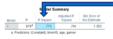
Predictive utility of regression model

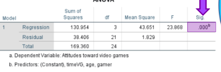
Do all predictors collectively account for a statistically significant proportion of the variance in the outcome variable?

sig = .000 therefore is significant

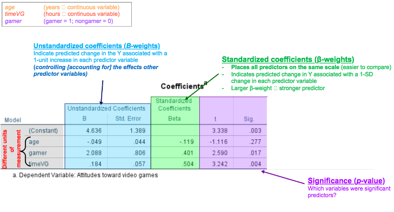
Standardized coefficients (β-weights)

Places all predictors on the same scale (easier to compare)

Indicates predicted change in Y associated with a 1-SD change in each predictor variable

Larger β-weight  stronger predictor

Unstandardized coefficients (B-weights)

Indicate predicted change in the Y associated with a 1-unit increase in each predictor variable

(controlling [accounting for] the effects other predictor variables)

Significance (p-value)

Which variables were significant predictors?

Equation:

Y' = b0 + b1X1 +b2X2 + b3X3

example:

y = 4.636(-.049)age+2.088(gamer)+(.184)hours

Standadised makes easier to combine ie. age is years, gamer is y/n, hours is time

Age not sig (.277)

Game, timeVG is (.017 and .004)

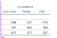
ZPP correlation FOCUS ON PART (in assignment)

Zero-order

bivariate Pearson’s correlation between predictor and outcome variable (r)

Partial

correlation between predictor and outcome variable (with the effects of all other predictors statistically removed [partialled out])

Semi-partial (part)

correlation between the predictor and outcome variable (with the effects of all other predictors removed [partialled out] only from the respective predictor)

We square the semi-partial values to calculate a the squared semi-partial (sr2)

sr2 = unique effect of each predictor

Percentage contribution of factor with everything else factored in

Partial correlation:

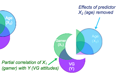
Semi-Partial correlation:

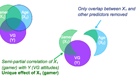
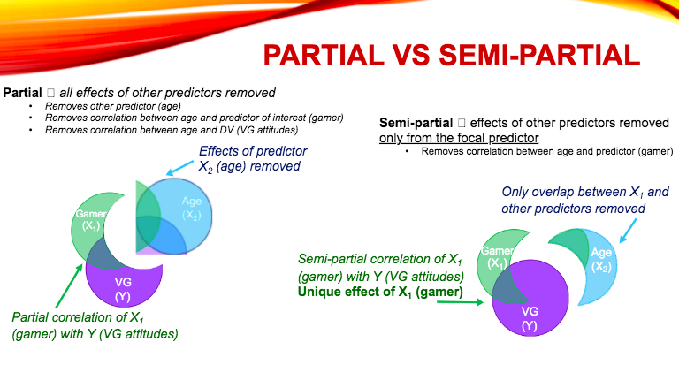
Semi-partial correlations

square semi-partial (sr2) statistic determines unique variance accounted for by each predictor

age (-.1162 = .0134) = 1.34%

gamer ( .2692 = .0723) = 7.23%

timeVG ( .3372 = .1135) = 11.35%

Pearson’s correlations between each predictor and DV

Negative correlation between age and video game attitudes (r = -.308)

Positive correlation between being a gamer and video game attitudes (r = .797)

Positive correlation between time spent playing video games and video game attitudes (r = .827)

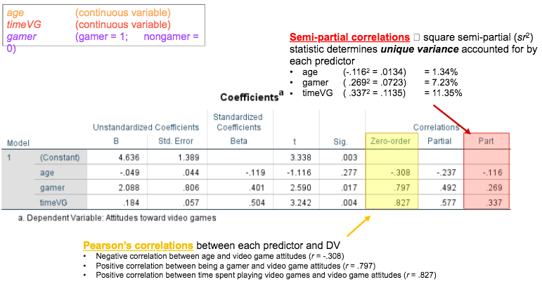
In diagram below:

Semi-partial correlations à square semi-partial (sr2) statistic determines unique variance accounted for by each predictor

•age (-.1162 = .0134) = 1.34%

•gamer ( .2692 = .0723) = 7.23%

timeVG ( .3372 = .1135) = 11.35%

- Individual unique part calculated

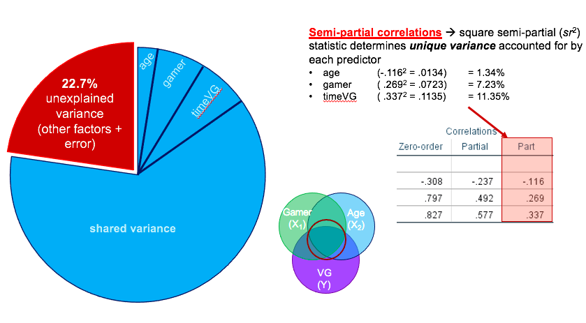
77.3% of the variance is explained by the predictors.

22.7% is error or other

Overall it is signfiant based on the significance level (.003)

y' = b0 + b1x1 + b2x2 + b3x3

y = 4.636 + (-.049)age + (2.088)gamer + (.184) timeVG

Correlations part

•age (-.1162 = .0134) = 1.34% = not sig (.277)

•gamer ( .2692 = .0723) = 7.23% = sig (.017)

•timeVG ( .3372 = .1135) = 11.35% = sig (.004)

We know that age, gamer and timeVG accounted for a significant proportion of the variance in attitudes to vg.

Example right up from worksheet:

a multiple regression was performed with gender, age, adn whether students completed maths B/C or not predicting attitudes towards this course. Table 1 displays the means, standard deveations and intercorrelations between teh four variables as was used in teh final regression. Gender was dummy coded where 1 was equal to being female adn MathsBC was dummy coded were 1 was equal to having done Maths B in high school. The regression model was found to be significantly different from zero, (F(3,65) = 4.06, p = .01. Altogether, our model accounted for 40% of the variability in attitudes towards this course. Examination of the B and Blong values and the sr2 values suggest that age was the strongest predictor of attitues towards this course accounting for 5% of unique variance in attitude towards this course. Respondents' age accounted for just under 5%of unique variance in the outcome, while gender accounted for 2%. Table 2 shows the unstandardised and standardised regression coefficients, squared semi-partial correlations and R2.

Página 7

Week 5

Basic recode:

recode variable_name (old_value = new_value) into new_variable_name.

Example: recode mathscourses (1,2 = 0) (3,4 = 1) (else=sysmis) into mathsBC.

Norms:

First, we normally assign the value of 1 in a dummy to the largest category. Second, we name the dummy for the group to which we have assigned the 1 score.

Important point: we always include into new_variable_name because we never want to modify the original data values.

Example, 2 statements, (1,2=0) (3,4=1), neatly cover the whole range of the mathscourses variable.

However, in practice, we can have variables with lots of categories (e.g. country of birth often finishes up with 50 separate values or more in a typical Australian sample if we include parents or grandparents). The beauty is that the syntax is exactly the same in form; we just include as many (old_value = new_value) statements as we need.

Example:

recode mathscourses (1,2 = 0) (3,4 = 1) (else = sysmis) into mathsBC.

Examples:

*(1 = 2) (2 = 1)

*simple one value swap (1 thru 3 = 1) (4 thru 6 = 2)

*ranges with minimum-maximum (1,3,5,7,8,12 = 1) (2,4,6,9,10,11 = 2)

*lots of non-contiguous values (1 = 5) (2 = 4) (3 = 3) (4 = 2) (5 = 1) (else = sysmis)

*reverse coding variable measured on a 1 -5 scale—same principle applies to all continuous scales (1 = 1) (2 = 0)

*creating a dummy from a variable scored 1-2. In regression, it matters that the values are 0 and 1. This is a very common manipulation (1 thru 3 = 1) (4 thru 6 = 0)

*creating a dummy from some sort of variable scored 1-6 (1 thru 3 = 1) (4 = 2) (5,6 = 3) (7 thru 9 = 4) (else = sysmis)

*we can mix and match all these as required we can put them on separate lines if it makes it easier to keep track of them and add white space too. e.g.,

(1 thru 3 = 1) (4 = 2) (5,6 = 3) (7 thru 9 = 4) (else = sysmis)

Página 8

Week 6

Correlations

Allow us to obtain an estimate of the population correlation

Reliability and validity estimates

Use in other analyses

E.g., basis of factor analysis

Calculate coefficient of determination

ie. variance occurance

Prediction

Cancer Risk

Predictors include:

Age, adiposity, alcohol consumption, medications, HRT, pregnancy, family history of breast cancer, ethnicity, etc

Criterion: Potential risk (range from low/average to high)

Is this 100% accurate? What is the “margin of error”

Regression and Prediction

If there is an association (or correlation) between Variables X and Y

if you know a value on Variable X (e.g., age), then you should be able to use it to make an educated guess about what the corresponding value on variable Y (e.g., cancer risk) will be

Regression gives life to the concept of correlation by using it for predictive purposes

In the language of regression,

Variable X in the previous example would be called the predictor,

and Variable Y the criterion

the predicted value of Y is referred to as Y’ (“y-prime”)

Sometimes referred to as (Y-hat)

if X and Y are perfectly correlated (r = 1 or -1), then prediction is easy…

just read off the scatterplot

but correlations are rarely ever perfect

However we can calculate a line that best represents the general relationship (or trend) of the data points

The “line of best fit” (aka the regression line) allows us to make predictions that are better than if we knew nothing about the relationship

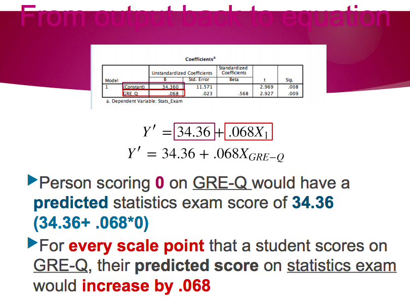
Y' = b0 + b1x1

·Y’ = predicted value of Y

b1 = slope of regression line · (rate at which Y changes with each 1-unit change in X)

b0 = intercept

(the predicted value of Y when X = 0)

Summary:

Correlations are used for multiple purposes

In this course we extend to the bivariate regression and use known associations to predict scores

We use the line of best fit (aka the regression line) to predict scores

Without knowing the association with other variables, our best guess on our criterion or outcome variable (our Y variable) is the mean of the Y

By using the regression equation that incorporates the value of the slope and intercept we can use the known associations with another variables to improve our predicted scores

Dichotomous Variables as Predictors

What if we had a record of all the students who attended every lecture during their graduate school statistics course and those that did not?

How would “attendance” correlate with statistics Exam performance?

What would the prediction be?

We can answer these questions using a special type of dichotomous variable – the dummy variable

Summary:

Regression analyses assume that both the outcome variable and the predictor variables are on a continuous scale

When we need to use dichotomous variables (i.e., categorical variables with two categories) we can create dummy variables by coding one category as one (1) and the other as zero (0)

We can then perform our regression analysis as usual

The value of intercept now has meaning and is the predicted value of the Y variable for participants who scored zero on the X variable

The value of the slope is the difference in the predicted score on Y for participants who scored one on X variable

You can calculate the predicted score on Y for these participants by simply adding (or subtracting if the slope is negative) to the intercept

Variance Explained

Bivariate regression

The special case of a single predictor and single criterion

An actual score comprises:

A systematic and

a random component

systematic = relationship w/ predictor

random = unrelated to predictor

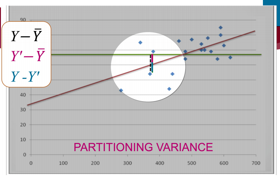
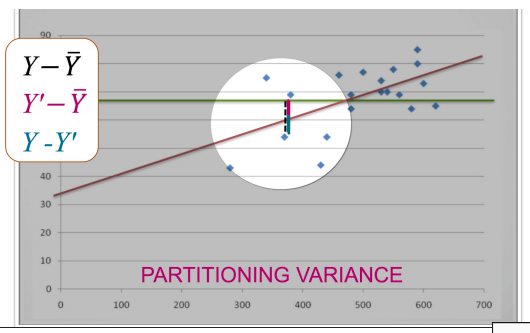
Total Variance

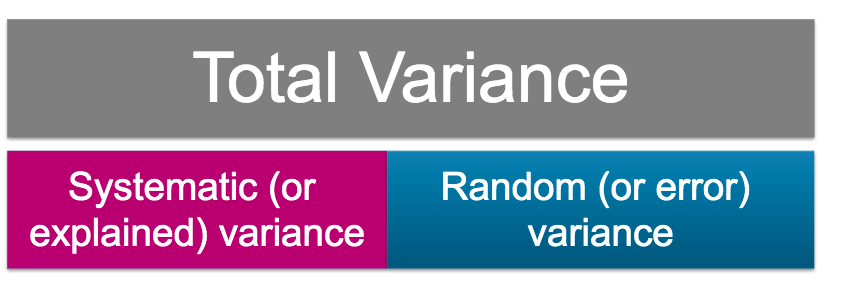
Total variance is the variance in the scores on the Y variable

We are interested in the deviations of all the scores from the mean of Y

This is represented by the black double-headed arrows

Systematic Variance

Systematic variance is the amount of the total variance accounted for (or explained) by the improvement in prediction by the regression line

This is the difference between each person's predicted score and the mean of Y

This is represented by the pink double-arrows

Random Variance

Random variance is the amount of variance leftover

This is the error or residual covered in the Prediction and Residuals mini-lecture in Week 4

This is simply the difference between people's actual scores and their predicted scores

This is represented by the blue double-headed arrows.

Sum of Squares

Sums of squares refers to the process that is part of calculating variance

Recall this equation from 1003PSY

In regression we care about explaining variance on the Y variable so we shall just change this a little

Recall to calculate variance you need to:

Calculate the deviation scores (score minus the mean)

Square the deviation scores

Sum them up

This part of the process creates a number called the Sums of Squares

Or more fully – the Sums of Squares of deviation scores

If I do the extra step of dividing by N I would have the variance. However, in regression we stop at the Sums of squares step

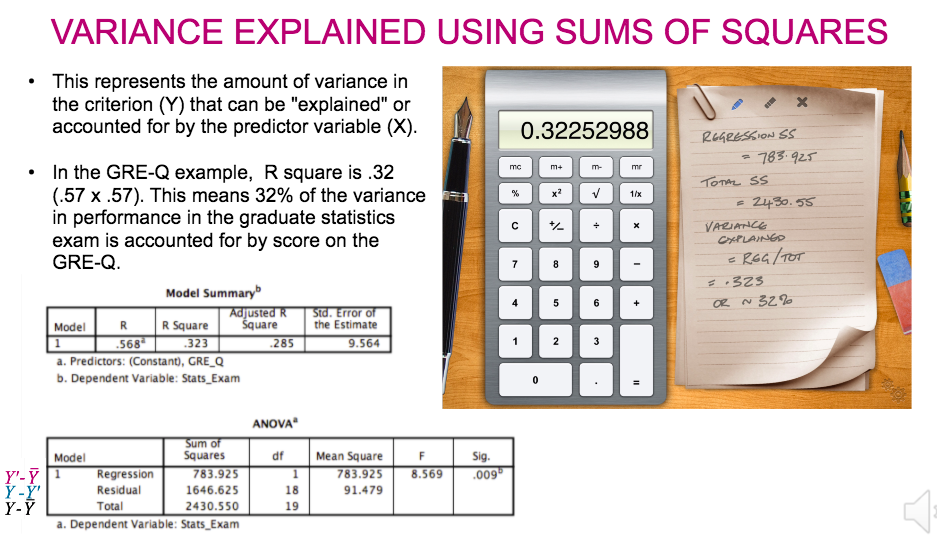
We can use the Sums of Squares approach to calculate the variance explained in our Y variable by our regression equation

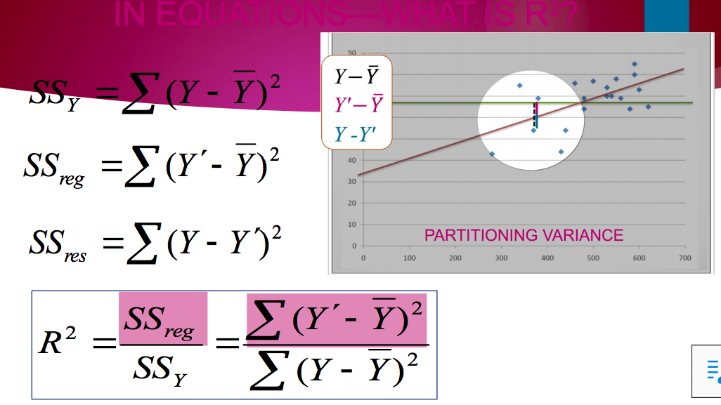
Total variance: SS for deviation scores from the mean of Y

- referred to as SSY or SSTOT

Systematic variance: SS for deviation of predicted scores from the mean of Y

- referred to as SSreg or SSregression

Random variance: SS for deviation of scores from predicted scores

- referred to as SSres OR SSresidual

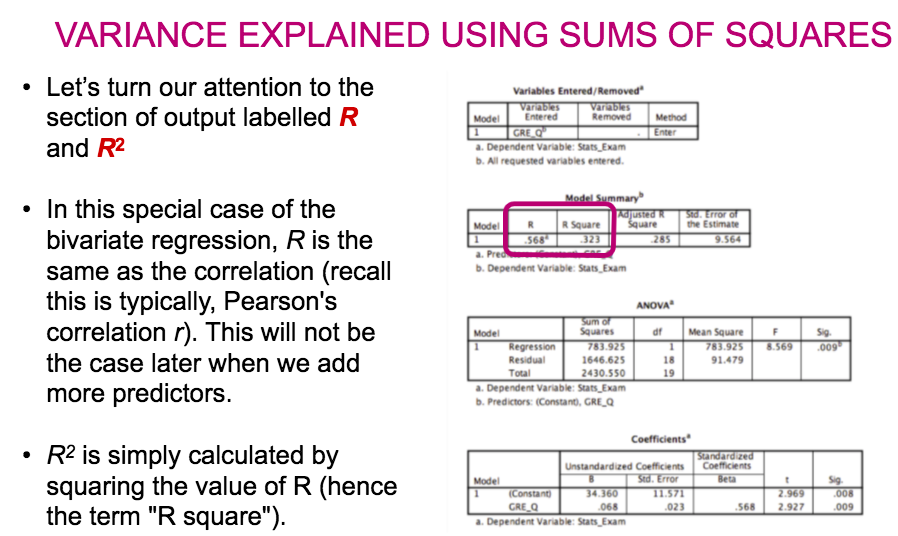
In correlation we can square the value of the correlation to obtain the variance explained

We could do the same in a bivariate regression as the Beta weight is the same as the correlation

However when we add in more predictor variables we cannot do this

Instead we will use two of our SS values and this formula.

R square is the proportion of the total variation of scores on the Y variable (SSy) that can be accounted for by the improvement in prediction by our regression equation (SSreg)

Página 9

Week 7

Multiple Regression

When we have > 1 predictor (X) variable, we simply need a way to combine them

The regression procedure expands seamlessly to do this…

Essentially, we extend the least squares procedure to estimate b0 and b1 and b2… bk to give us the best possible prediction of Y from all the variables jointly

This type of regression might be referred to in some texts as OLS, Ordinary Least Squares Regression

B-weights in multiple regression

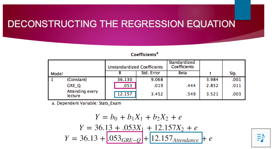
the b-weights are the numbers by which we multiply (i.e., weight) each X to make a composite X with all the information from the separate Xs in it • the b-weights are the numbers by which we multiply (i.e., weight) each X to make a composite X with all the information from the separate Xs in it

Are partial slopes:

each b tells us how much change in pred. Y there will be for a change of 1 in that X when all the other Xs are held constant

This gives us a clue as to how much each X is related to Y when considering the interrelationships among the Xs • better than looking at correlations among all variables as these are not corrected

Standardised Weights

Beta (β) weights

As for b weights but for standardised solution

Intercept = zero and drops out of equation

Give a measure of slope in standardised units

This aids in comparison but is not importance as is misleadingly stated in some sources

Variance explained

Significance testing

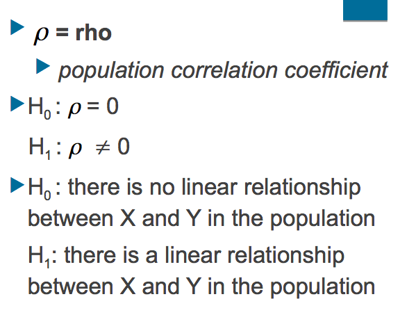
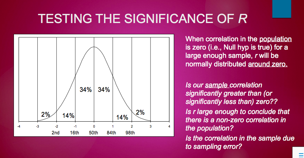
R significance

r describes the linear relationship between two variables in a sample

usually want to make inferences about the relationship in the population

is r large enough to conclude that there is a linear relationship between the variables in the population? or

is the correlation in the sample due to sampling error?

rho

Summary

Just as with our other analyses like the t test we check for significance of our overall R and for our b weights

The correlation in the population is referred to as  (Rho)

We use the same concept of sampling distributions as we used with means to test whether the correlation or the b weight in our sample is significantly different from zero

In addition to testing whether there is a significant association between our predictors as a group (aka a linear combination; the regression equation) by looking at R we also test the significance of each predictor while controlling for all other predictors by looking at the significance of the b weights

Proportion of variance

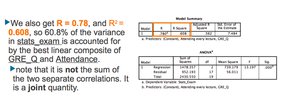
In correlation, r 2 = proportion of variance shared by X and Y, i.e., the two correlates—overlap

In regression, this still holds of course, but…

… now, we speak of the amount of variance in Y accounted for by X (either a single predictor or the set of predictors)

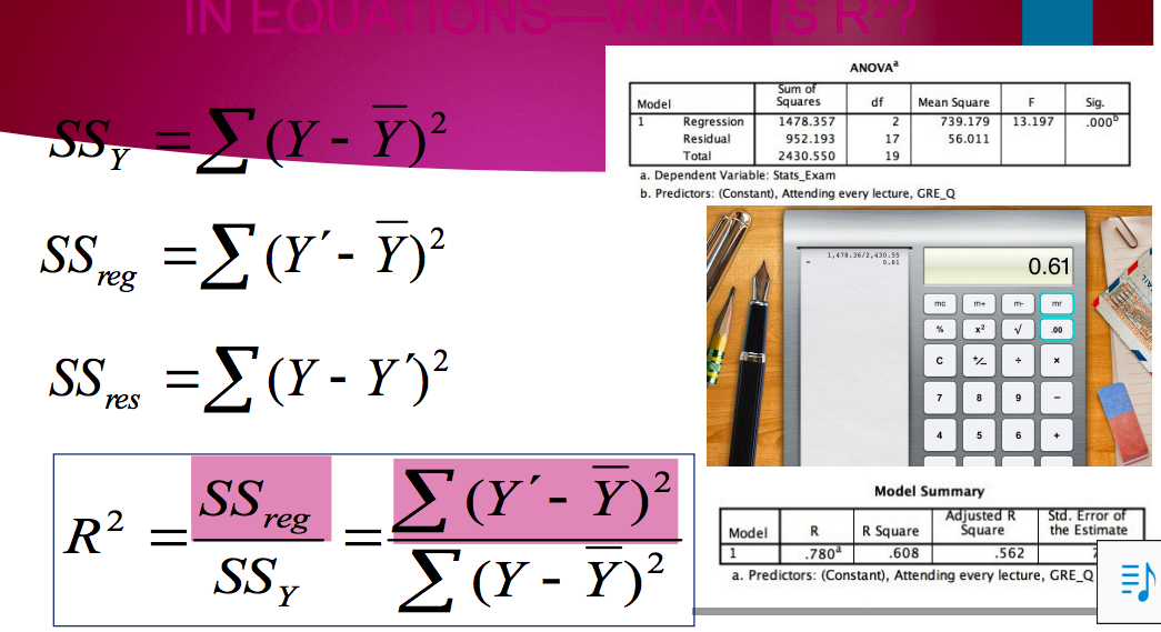
Multiple R2 is variance in Y accounted for by Xk

usually referred to simply as R2 Not specific to any one single X, it is for the set of them.

The regression equation is also referred to as the Model

we check the value of R2 in the Model Summary box in the SPSS output

Semipartial correlations—sr and sr2

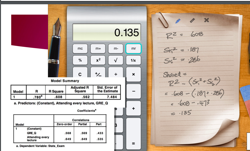
Relationship between Xk and Y when all other predictors partialled out of only Xk .

Good indicator of the unique relationship between Xk and Y

Always squared (i.e., sr2 ) to give proportion of unique variance in Y accounted for by Xk

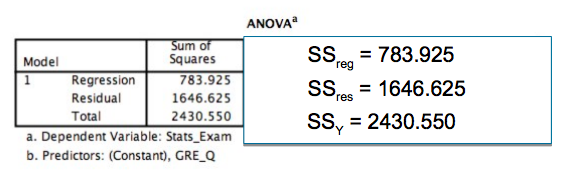
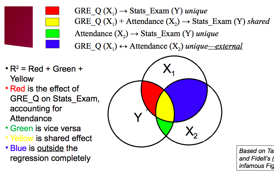
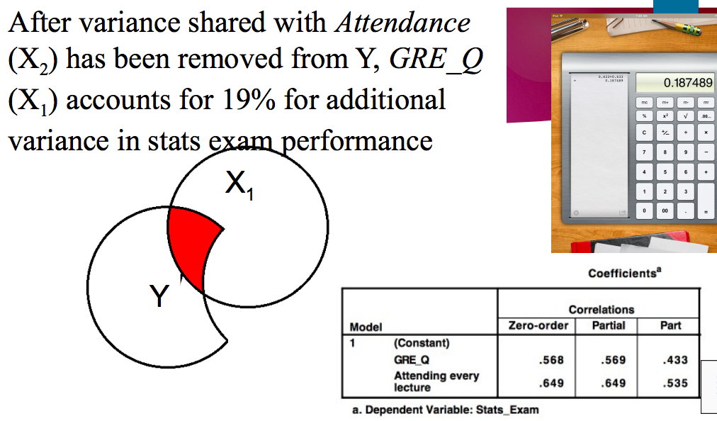
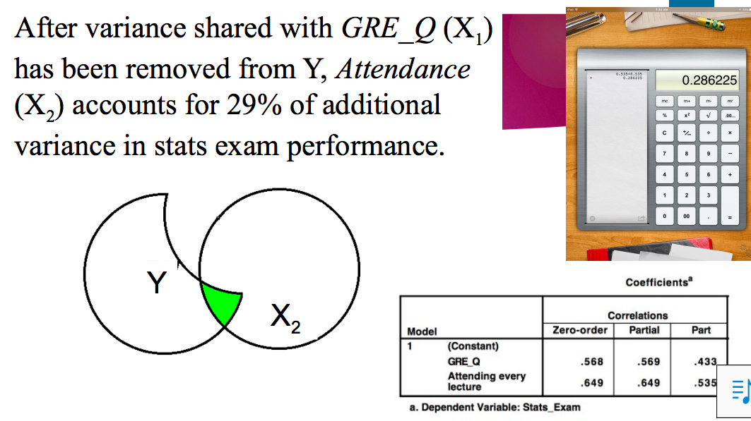
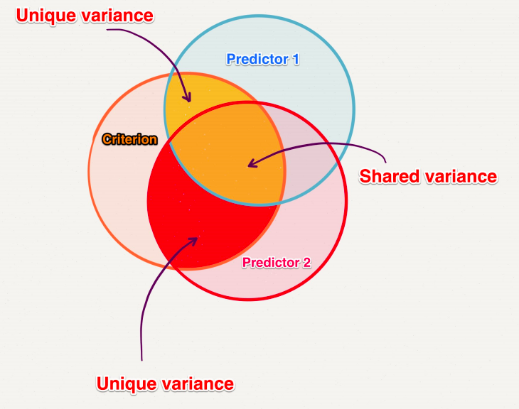
Shared Variance is the difference between the combined unique variance (sr2 GRE_Q +sr2 attendance) and total variance explained (R2 )

Summary

R square refers to the variance in the Y variable explained by the linear composite (aka regression equation or model)

In multiple regression we want the variance explained by each predictor variable after controlling for the other predictor variables

We call this unique variance and is represented by squared semipartial correlations

The difference between total variance explained (R2 ) and unique variance is shared variance

We can look at the unique variance to better understand the strengths of the relationships between our predictor variables and the outcome

Página 10

Week 8

Regression assumptions

Regression is a powerful analytic approach that requires consideration of underlying assumptions

Assumptions are made with regard to the residuals  We assume normality of residuals, homoscedasticity, independence of residuals, and linearity

These assumptions are tested by requesting additional information in our syntax

Violations of assumptions may reflect skew, outliers, and/or non-linear associations

Violations

When assumptions have been violated, short of re-evaluating our model selection and our analysis plan, we turn to the state of the variables

Are the vars badly affected in terms of normal distribution?

It may be that addressing normality, where possible, may fix the violation

Q. If they are so, why are the variable/s nonnormal?

Skewness

Measurement? Structural property of data (e.g., frequencies)

Outliers

Curse of sampling (worse for small N)? Truly member of another population caught in our net?

Some advocate a strategy in which the analyst blindly checks all variables for skewness and kurtosis and routinely transforms any that are nonnormal

This is a problem if it is perceived to be a sort of insurance against later woes.

In fact, if the residuals and the residuals plots look OK (see Tutorials) then you don’t need any further transformations.

However, for the assignment still check skew, outliers, etc even if the residuals look ok.

You have to look at the data and have some idea of where they came from!! The data don’t know this themselves.

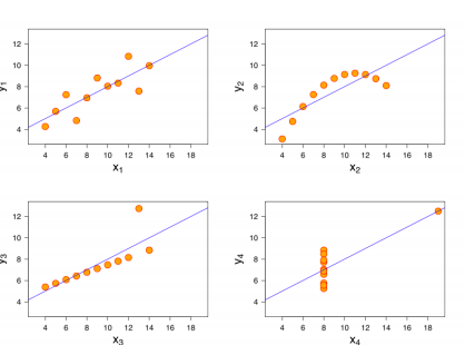
Anscombe's Quartet

Data sets famously derived by Frank Anscombe

These illustrate how characteristics such as nonlinearity and outliers can exert serious distortion on (our interpretations of) correlation (and regression) statistics

Most importantly, they point out that we cannot have confidence in statistics without examining the form (visually!) of the underlying data

They also show us that blindly chasing assumptions in regression could be as pointless without examining the data and trying to understand why it is distributed the way it is.

These illustrate how characteristics such as nonlinearity and outliers can exert serious distortion on (our interpretations of) correlation (and regression) statistics. Most importantly, they point out that we cannot have confidence in statistics without examining the form visually of the underlying data.They also show us that blindly chasing assumptions in regression could be as pointless without examining the data and trying to understand why it is distributed the way it is.

The four dataset are created to all have the same mean, variance, correlation, and regression equation

Dataset 1

The scatterplot from Dataset presents a very nice linear pattern of scores that evenly lie near the regression line. However, the scatterplots from the other three datasets look very different even though the descriptive statistics would be identical.

Dataset 2

Below I have superimposed the scatterplot based on the second data set. Drag the line to show the differences between the scatterplots based on the two datasets. Recall that this dataset has the identical (to 1 decimal place) means, variances, correlation, and regression equation. See how by looking at the scatterplot that we have a curvilinear association !

Dataset 3

Below I again have superimposed the scatterplot based on the third dataset over the original data. Once again I remind you that this third dataset has the identical (to 1 decimal place) means, variances, correlation, and regression equation ! See how by looking at the scatterplot that we can see that we have an outlier on the Y variable

Dataset 4

Finally , I have superimposed the scatterplot based on the fourth dataset over the original data. Reminding you yet again that this third dataset has the identical (to 1 decimal place) means, variances, correlation, and regression equation ! See how by looking at the scatterplot that we can see that we have an outlier on the X variable.

More regression assumptions

Regression assumptions are actually made about the residuals (i.e., the e in Y = b0 + b1x1 + e)

We can’t do anything directly to the error as it is what is left over after the line (i.e., predicted Y) has been fit

regression will still “work” for nonlinear relationships but interpretations of parameters on face value may be meaningless

Normality

residuals (errors) are normally distributed with mean = 0

often said, centred around 0 (zero)

Homoscedasticity

constant variance of residuals (across predicted scores)

Independence of errors

The residuals are uncorrelated with Y

linearity of the relationship

If we want the benefits of regression to answer our RQ, we have to pay the costs of ensuring that our data meet the underlying assumptions

MR Partitions

We predict the actual ( Y) score from the Xk predictors—what Y “should” be

A predicted score (Y′) is derived from this

Unless the correlation is perfect, Y ≠ Y′

Y - Y′ = e

e = error/residual

= whatever leftover in Y that Y′ doesn’t account for

Y = Y′ + e

Y = Predicted + Residual

Each person “has”:

an actual (Y) score

a predicted Y′ score

a residual “score”

Residuals

If the regression equation has underestimated the actual score, the residual will be positive

If instead the true score was overestimated, the residual will be negative

The assumptions are about the residuals but we use the standardised scores and regress the standardised residuals on the standardised predicted score. • We don't need to do this separately we use syntax and add this to the multiple regression syntax

The residuals can take on distinctive patterns if there is something systematic and amiss.

If there were only true score and random error in our data and we hadn’t omitted any important predictors of our outcome, we would expect nice neat, normally distributed residuals centred around zero…

Anything else means that there might be a problem

Homoscedascity

When we have our residuals correlated with predicted scores

And we have random error (i.e., error is independent of association with the criterion)

And we haven't left out important predictors

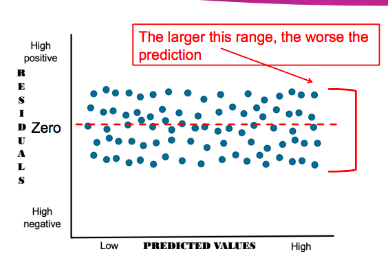
We should have a rectangular shape

We have met the assumption of homoscedascity

The residuals should be evenly scattered above and below zero

The range of residuals around zero should be narrow

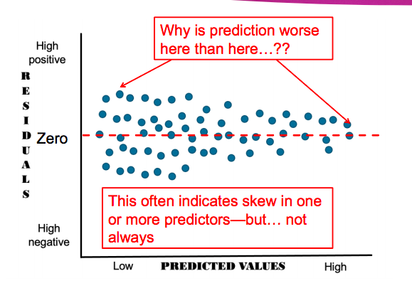
If however our residuals look like a funnel or a fan then this suggests that we have not met the assumption of homoscedascity

The distribution of residuals across the range of predicted values of Y is not even

If however our residuals look like a funnel or a fan then this suggests that we have not met the assumption of homoscedascity

The distribution of residuals across the range of predicted values of Y is not even

How do we address violations

Short of using a different statistical procedure entirely, we have 2 courses of action open to us

We may find one or more outlying data points on one or more variables that are unduly influencing the regression analysis and leading to potentially erroneous conclusions

One or more predictors may deviate greatly from normality—skewness and kurtosis. Again, this may lead to errors

a) In this case, we generally apply one or more transformations of the data (in turn, not concurrently).

b) We replace the actual variable with the transformed one in the regression.

c) Certain transformations may help alleviate skewness (caution, hit and miss!)

Outliers and transformations are covered in the next topic and in the tutorials

Regression is a powerful analytic approach that requires consideration of underlying assumptions

Assumptions are made with regard to the residuals

We assume normality of residuals, homoscedascity, independence of residuals, and linearity

These assumptions are tested by requesting additional information in our syntax

Violations of assumptions may reflect skew, outliers, and/or non-linear associations

Página 11

Week 9

Non-parametric tests: Spearman's Rho

All of the tests we have considered up to this point have involved:

estimating population parameters

assumptions about the shape of the data

assumptions about the scaling of the variables

Estimating Population Parameters

parametric tests involve the estimation of at least one population parameter

e.g., t-test uses sample variance to estimate the population variance

non-parametric tests do not— hence the name

Assumptions about the shape of the data

Parametric tests also make assumptions about the distribution of the population from which the data were randomly sampled all the tests we’ve looked at so far have all assumed that the data is normally distributed

e.g., t-test assumes that the sampling error is distributed normally around m

non-parametric tests do not make a priori assumptions about the specific shape of the distribution—hence they’re also known as distribution-free tests

Assumptions about the scaling of the test

Parametric tests assume the outcome variable has been measured at interval or ratio level

Non-parametric tests do not

Non parametric tests

Advantages

They do not require assumptions of normality and homogeneity of variances (severely skewed data can be analysed with nonparametric statistics)

Ideal for analysing data from small samples (small samples are often skewed and can’t be rescued by the central limit theorem)

Generally easier to calculate--require less computation

Use of ranks reduces effect of extreme outliers

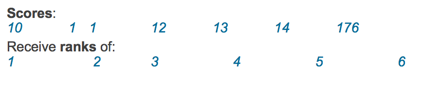
Explaining Ranking

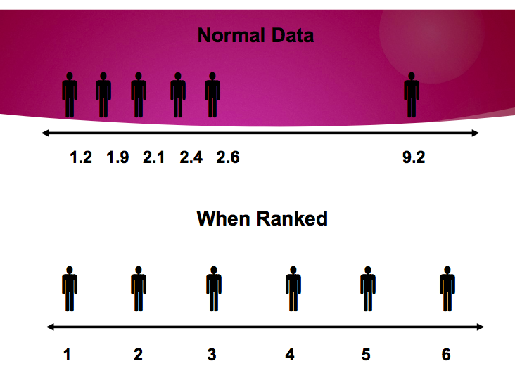
ranking merely involves the ordering of a set of scores from the smallest to the largest

the smallest is given the rank of 1, the second smallest the rank of 2 … the 50th the rank of 50

Why rank?

it provides a standard distribution of scores with standard characteristics

Spearman Rank-Order Correlation Coefficient (or Spearman's Rho)

Pearson’s correlation coefficient r is based on assumptions:

interval or ratio data,

X and Y are normally distributed, and

a linear relationship between X and Y

So we assume a bivariate normal distribution based on interval or ratio scales

Spearman's rho (rS ) is calculated using Pearson’s r formula - the difference is that the data is ranked

this is handy if:

The data naturally falls in ranks

there are extreme scores in your sample

there is a monotonic relationship between the variables

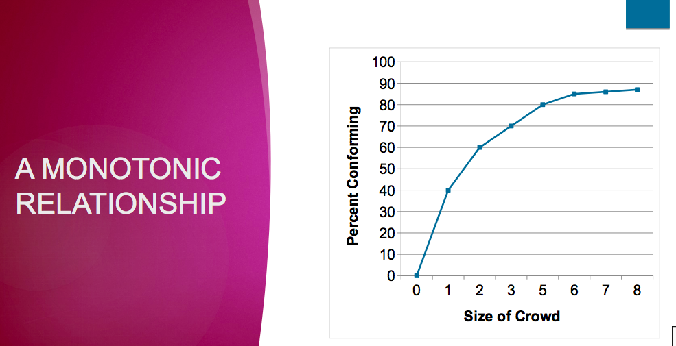
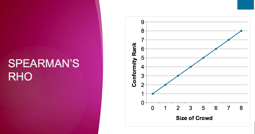
another benefit of Spearman’s rho is that it can be used when you have two continuous variables, but one (or both) is badly skewed due to extreme scores

The Null Hypothesis

The goal of any non-parametric test is to establish overall differences between two (or possibly more) distributions, not to identify the differences between any particular parameters

as a result, H0 is more general

samples come from identical populations, not just populations with the same mean

rejecting H0 means that populations differ (perhaps not just on the basis of their central tendency - i.e., the mean)

Summary

Parametric tests involve estimating population parameters, making assumptions about the shape of the data and assumptions about the scaling of the variables

Non-parametric tests do not

Ranking is one approach used by non-parametric tests

Spearman's rho can be used to calculate correlations between variables that has natural ranks, there are extreme scores in your sample or there is a monotonic relationship between the variables

While fewer assumptions are required to be met non-parametric tests are generally less powerful than parametric tests.

Point serial Correlation

Pearson’s r is appropriate for describing linear relationships between two continuous variables

if one variable is genuinely dichotomous, score one level of that variable as 0 and the other as 1 (or 1 and 2, or any two numbers)

compute correlation using Pearson’s r formula

referred to as the point-biserial correlation (rpb)

Interpretation of point serial correlation

absolute value of rpb reflects strength of the relationship

but the sign of the correlation depend on scoring (0 or 1; or 1 and 2)

r 2 pb interpreted the same way as r 2

test for significance in same way as for Pearson’s r

rpb and t

Alternatively, we could examine the relationship between a dichotomous and a continuous variable using an independent groups t-test

Result of test of significance of r pb and t-test will be identical

Summary

A point biserial is a special case of a correlation with one continuous variable and one dichotomous variable

The point biserial is interpreted the same a Pearson's correlation

The t value and significance of a dichotomous predictor in the regression output is the same as if the analysis is tested as a t test.

You can use the regression equation to calculate the mean of the two groups in the dichotomous variable just like in a t test

Página 12

Week 10

Chi Square

Chi square is a test used on frequency data

Chi square allows us to test research questions with categorial data

Categorical

Nominal

measures are just names for things e.g. gender

Continuous

Ordinal

measures the rank ordering of something e.g. 1st/2nd place

Interval

equal differences between scores can be treated as equal units e.g. degrees C

Ratio

interval scale with a true zero point e.g. length

Chi Square

In the one-way chi square we can ask research questions like

Are people/things distributed evenly across the categories of the variable? We can also test out other distributions (we will come back to this)

Chi Square Test:

Chi-square analyses involve working out the expected likelihood of something happening (what frequencies you should get if the null hypothesis is true) and comparing it with the observed frequencies (what frequencies you do get)

Chi-square tells you how well the expected and observed frequencies match … for this reason it is often referred to as a test for “goodness of fit” (do the observed frequencies “fit” the expected frequencies?)

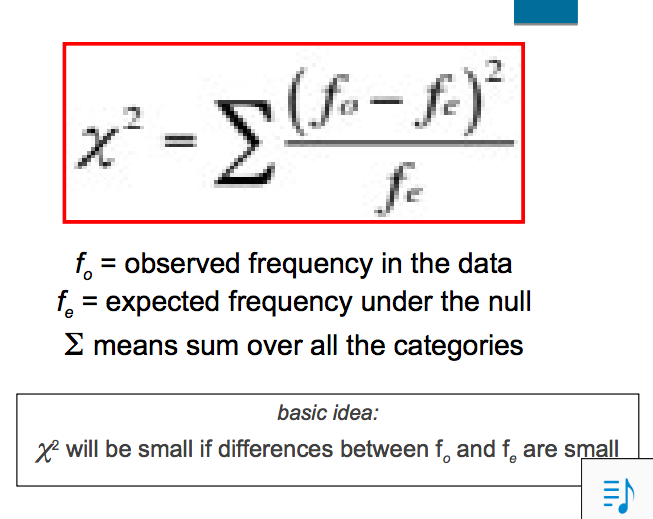
Calculation of chi (x2)

f o = observed frequency in the data

f e = expected frequency under the null

 means sum over all the categories

x2 will be small if differences between fo and fe are small

Expected Frequencies

what do we expect? what is the null?

uniformly distributed -> equiprobable distribution

distributed in accord with theory

distributed in accord with previous observed frequencies

normally distributed

COMPARING OUR OBTAINED STATISTIC AGAINST CHISQUARE DISTRIBUTION (NULL)

H0 : in the population, the distribution across categories = expected frequencies

Therefore, any discrepancy = chance

How big can the discrepancy be before we reject possibility of H0 being true?

Use the standard cutoff of .05

i.e., a discrepancy large enough that less than 5% of samples exhibit it when the null hypothesis is true.

SAMPLING DISTRIBUTION OF X2

x2 is a family of distributions dependent on df

however, df depends on number of cells, not number of participants

• df = k – 1

X2 values always positive

can increase x 2 obt by increasing sample size

e.g., could double x2 value by doubling sample size but x2 crit remains the same

In practice

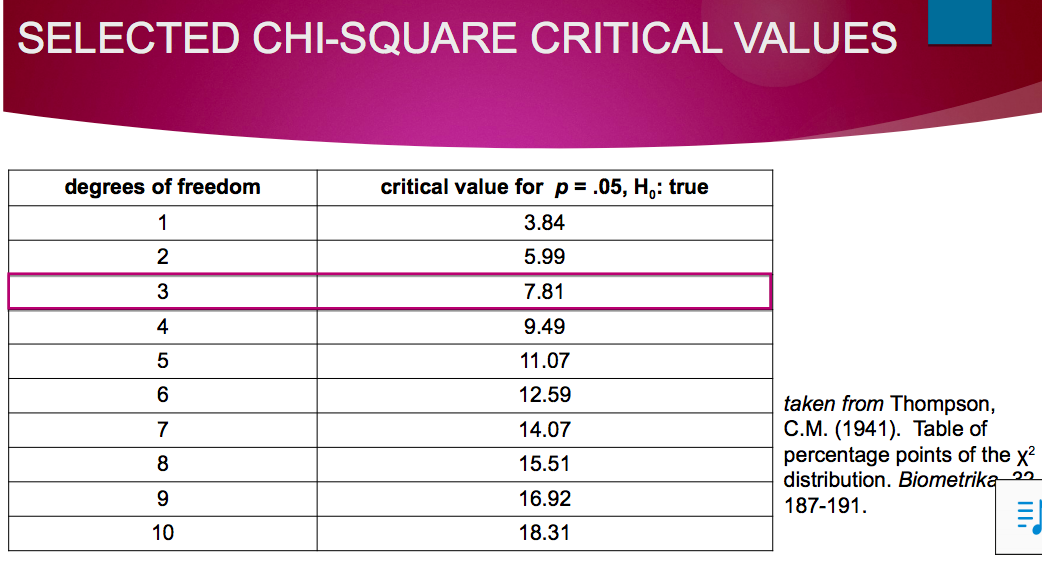
We only need the critical value of chi square for the degrees of freedom in our study

• critical value = value that marks .05 region under the null

Calculating df for a one-way chi square

df = k – 1, k = number of categories

Four categories of chupa chup flavour

k = 4, so the df = 3

Expected frequencies

for some variables, simple equivalency distributions under chance might be a useful benchmark against which to test

e.g., marketing and popularity of choice

in other cases, we might have a more plausible expected distribution against which to test our sample

that is, we already know that the categories won't be exactly equal

what do we expect? what is the null?

uniformly distributed -> equiprobable distribution

distributed in accord with theory

distributed in accord with previous observed frequencies

normally distributed

Summary

Chi square tests research questions for nominal (aka categorical) data

Chi square tests use frequency data

The one-way chi square test is also referred to as the Goodness of Fit chi-square

The chi square compares obtained frequencies to expected frequencies as stated under the null hypothesis

To test the significance of a chi square, the obtained value is compared to the critical values in the chi square distribution

The degrees of freedom in chi square depend on the number of categories – not the sample size

The one-way chi square can specify different null hypothesis

A common null hypothesis is the equiprobable distribution

TWO-WAY CHI SQUARE AKA CHI SQUARE TEST OF INDEPENDENCE

Relations between variables can also be tested with the chi-square test

Good news: formula for chi-square the same

Less than good news: new formula for fe

you’ll love it in the end

The null hypothesis in this case is that the two variables are distributed independently

referred to as x2 test of independence

Also x2 contingency

One variable must not depend on another

two variables are considered to be independent when the frequency distribution for one variable has the same shape for all levels of the second variable

i.e., salary is independent of gender

Summary

One-way chi-square (aka goodness-of-fit)

One-way: generally, does the observed data fit the model?

Two-way chi-square (aka test of independence)

Two-way: are the two variables independent ?

test two somewhat different questions

THE LOGIC OF THE TEST OF INDEPENDENCE

By ignoring the frequencies within the body of the table and just focusing on the marginals, we are viewing the data from the perspective of the null (H0 )

if H0 is true, then the marginals are all we need to understand the variables as they would be distributed independently

How do we obtain the necessary expected frequencies?

we use the frequencies expected under independence

If the variables are independent, the relative proportions of those who passed/failed (70:30) should be mirrored in each level of the Attendance variable

i.e., 70% of those with perfect attendance would pass and 30% would fail and

70% of those with less than perfect attendance would pass and 30% would fail

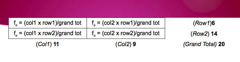
We only need the marginal totals and the grand total

the expected frequencies (i.e., fe ) represent the null

For each cell: f e = (column total x row total)/grand total

We have essentially duplicated the table and replaced the obtained frequencies (i.e., our actual data) with the expected frequencies that represent the way the data ought to look under the null (i.e., when H0 is true)

Two-way chisquare

for a two-way chisquare, df = (Rows – 1)(Columns – 1)

in our case: df = (2 – 1)(2 – 1) = 1

Critical value for df = 1 is 3.84 p = .05, H0 : true

Our obtained value of chi square of 7.02 is larger than 3.84.

Therefore we reject the null hypothesis of independence and conclude that our sample represents a population in which class attendance and grade (fail/pass) are associated i.e., not independent

Summary

The two-way chi square tests the association between two categorical variables

The two-way chi square is also referred to as the Test of Independence

The expected frequencies of the two-way is set to test for independence of the two variables

The calculation of expected frequencies involves the marginal totals and the grand total

The obtained chi square is tested against the chi square distribution

The calculation of degrees of freedom involve the number of categories of both variables, not sample size

Calculating by hand is better than SPSS when you only have the cell means

ASSUMPTIONS OF x2

independence of observations

a participant must fall in one and only one category – they cannot be counted twice thus you cannot use chi-square on repeated measures designs

special forms of tests exist to test out such relationships but these are well outside the scope of 3003PSY

size of expected frequencies

all expected cell frequencies should be at least 5, if they aren’t you shouldn’t use a x2 test

small expected frequencies produce few possible values of chi-square obtained x2 but we compare to continuous distribution

the greater the degrees of freedom, the more lenient this requirement

Inclusion of non-occurrences

computations must be based on all participants in the sample

Limitations

Not really a limitation but this is restricted to ≤ 2 vars

larger designs routinely analysed using multivariate generalisations of these approaches that are largely based on log-linear models and are best covered in their own course!

just as MR is to simple regression, log-linear models are to chi square

Effect size

a significant x2 does not indicate strength of the relationship 2 does not indicate strength

if your sample size is large enough, sometimes very small effects will be detected as significant

a significant x2 a significant c does not indicate strength of the relationship

if your sample size is large enough, sometimes very small effects will be detected as significant if your sample size is large enough,

but we can convert x2 to a measure of association that tells you how big the effect is

EFFECT SIZE: PHI

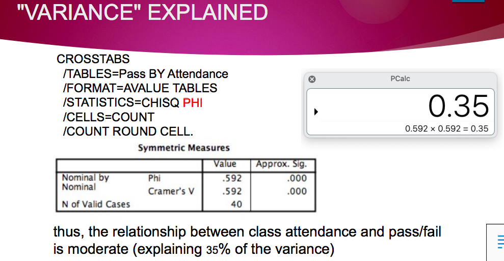
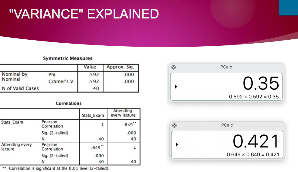
phi (f) for 2 x 2 chi sqaure

interpreted as Pearson r

correlation between two variables, each of which is a dichotomy

if chi-square is significant, so is phi

can be interpreted in terms of Cohen’s conventions.

Although is a measure of association between two variables, rather than effect size, these concepts are related.

so, for example, if  = .50 – you could say that there is a moderate level of association between the two variables.

or, for example, if  = .65 – you could say that there is a moderate to high level of association between the two variables.

Cramer’s phi (fc ) a generalisation of phi to r x c tables (will also work for a 2 x 2 table, as k – 1 will = 1)

Interpret the same as Phi

Summary

Chi square has several assumptions and limitations

Independence of observations

Expected cell frequencies of at least 5

Inclusion of non-occurrences Can only be used with 1 or 2 variables

As DFs are based on number of cells, sample sizes has a strong influence on the obtained chi square and by extension significance

Phi is the measure of association between categorical variables in a 2 x 2 chi square

Squaring Phi provides variance accounted Cramer's Phi is used for chi squares with > 2 x 2

Página 13

Week 11

Surveys and Causation

•Determinations of causation are based on three criteria

1.The constructs need to covary;

1.There must be temporal precedence, and;

1.No confounding factors (i.e. alternative explanations need to be ruled out).

Temporal Precedence

•In cross-sectional research, temporal precedence can never be directly empirically tested

•The ‘causal’ direction is inferred by allocating a variable as the criterion (DV), and others as predictors (IVs). This suggests the IVs ‘cause’ the DV.

•Theory and previous empirical findings are used to justify the direction of the statistical analysis.

Panel Design

•Panel designs are the gold-standard technique in longitudinal survey research.

•In a panel design, the same participants complete the same questionnaire over multiple time points.

•This ensures that both the predictor and criterion variable are measured at multiple time points.

Stability and Change

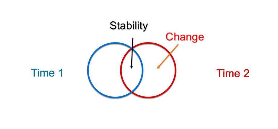
Stability: The degree of consistency in scores, means, or rank orders from one time point to another.

•A large autoregressive coefficient can mean one of two things*:•

1.Individuals do not change over time.

2.Individuals uniformly increase or decrease over time.

*There are other, more complex and less common explanations, that are not covered in this course.

Change: The degree of fluctuation in scores, means, or rank orders from one time point to another.

•In what ways and how much do things stay the same over time versus how much do they change. Often tested as baseline (the initial measurement) to re-test.

DIRECTION OF THE ASSOCIATION

•Uni-directional relationship:

•There is a clear direction in the relationship between the predictor and criterion variable.

•A uni-directional relationship in a well-designed longitudinal study provides support for temporal precedence

Bi-directional relationship

•Occurs when the predictor variable is related to the criterion variable, and the criterion variable is related to the predictor variable.

•In this instance, it is not possible to conclude that one variable occurred prior to the other, so temporal precedence cannot be determined. Rather both variables ‘cause’ one another…

Analysis of Longitudinal Survey Data using Regression

Simplex Designs

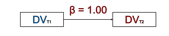
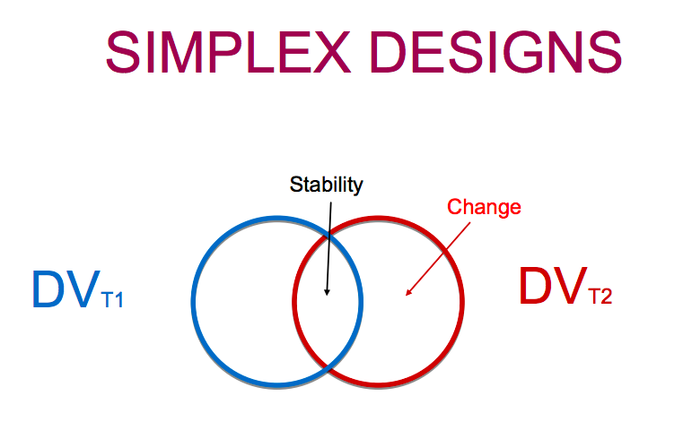
•Simplex designs, also known as autoregressive designs, involve regressing a variable on itself across time.

•In other words, the measurement of a variable at time 1 should predict time 2 (i.e., stability).

•This type of model is called autoregressive as the values of a scale are automatically regressed onto the same scale.

•This type of analysis allows researchers to explore the stability and change in one construct.

Simplex Design

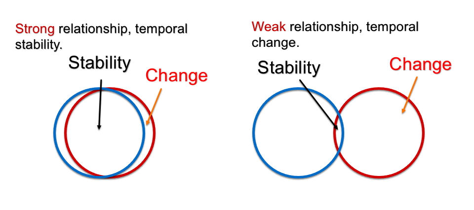
•A perfect association between the two time-points indicates that individual’s relative standings on the construct have not changed.

The rank-order of the participants remains the same. Participants with high T1 scores, will have high T2 scores (i.e., there is a high degree of stability from T1 to T2)

Across each of these explanations, the rank-order of the participants have not changed. Therefore, on a between-participant level (inter-individual), there is stability

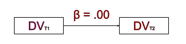
Simplex design

A small or zero association between the two time-points indicate that individual’s relative standings on the construct have changed dramatically (i.e., there is a lot of change from T1 to T2).

LONGITUDINAL CORRELATIONS

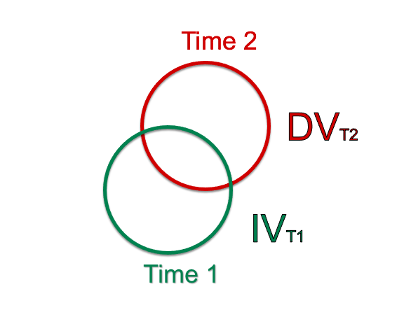
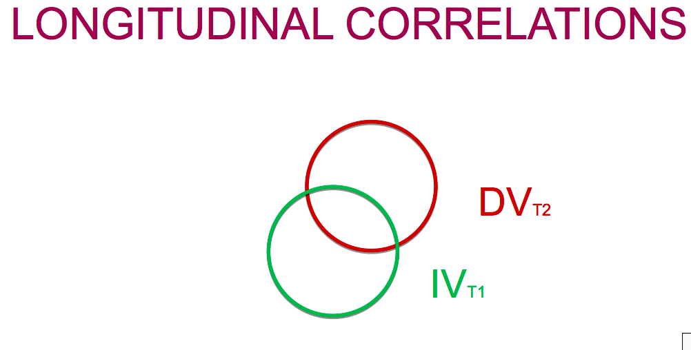
•Longitudinal correlations examine the relationship between the IV at time 1 and the DV at time 2.

•Similar to the correlations and bivariate regression techniques covered in this course, only two variables are analysed.

LONGITUDINAL CORRELATIONS

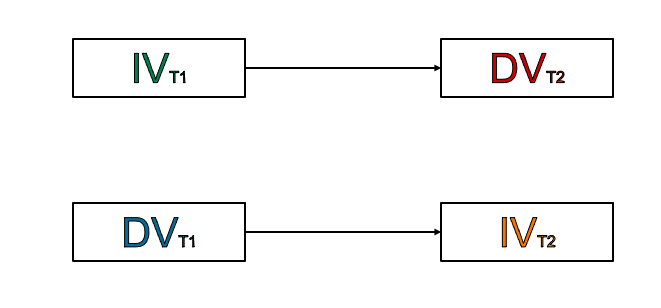
•In order to examine temporal precedence, researchers can run two separate longitudinal correlations.

•If the relationship between IV at time 1 and DV at time 2 is significant AND the relationship between the DV at time 1 with the IV at time 2 is not significant, it can be argued that temporal precedence has been found.

•If both analyses are significant, it may indicate a bi-directional relationship.

Weaknesses

•This analysis does not account for correlations between variables at each time point.

•Does not account for the stability in a construct.

There is no indication of the stability or change in the construct over time.

•The combination of these limitations ensure researchers cannot rule out that the relationship between T1 and T2 is simply due to a cross-sectional relationship.

Summary

We use longitudinal designs when collecting survey data in order to test for temporal precedence

We collect data for our variables at each time point

Simplex designs allow us to establish stability and change

Strong autoregressive associations show stability; weak autoregressive associations show change

Simplex designs do not establish temporal precedence

uLongitudinal correlations have been used to try to establish temporal precedence but not stability nor change

RESIDUALISED LONGITUDINAL REGRESSION

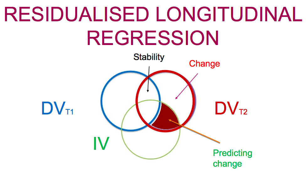
To address the limitations of longitudinal correlations, researchers can ‘residualise’ the DV.

This is done by entering the score of the DV at time 1 into the analysis.

As a result, the correlation between the DV across two time points is considered (i.e. the stability), and then statistically removed from the analysis

• This process allows researchers to ‘predict change.’

By entering the DV at time 1, the unique variance remaining in the DV at time 2, reflects the change in the construct over time

Residualised Londitudinal Regression

Strengths

The correlations between variables at T1 statistically controlled for.

The stability of the DV is accounted for.

Consequentially, this analytical technique allows a researcher to predict change (in other words, find a longitudinal effect).

Weaknesses

• Temporal precedence is still not identifiable because there is no test for bidirectional relationships.

Summary

Residualised longitudinal regression combines the strengths of the simplex design and the longitudinal correlation In this design the DV measure at T1 is entered into the analysis along with the IV to predict the DV measured at T2

This partitions the variance in the DV measured at T2 into variance shared with the DV measured at T1 (stability) and unique variance – the “residualised” variance (change)

The IV can then be used to predict change in the DV

This approach is limited in testing for temporal precedence as it cannot test for bi-directional relationships

CROSS-LAGGED MODELS

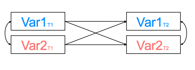
In cross-lagged models, the two measures serve as both the independent and dependent variable.

In this analysis, there is more than one DV

Cross-lagged models combine two residualised longitudinal regressions into the same analysis.

Thus, the stability of the construct is statistically removed, allowing each variable to predict the change in the other variable.

This technique allows an investigation of bidirectional effects.

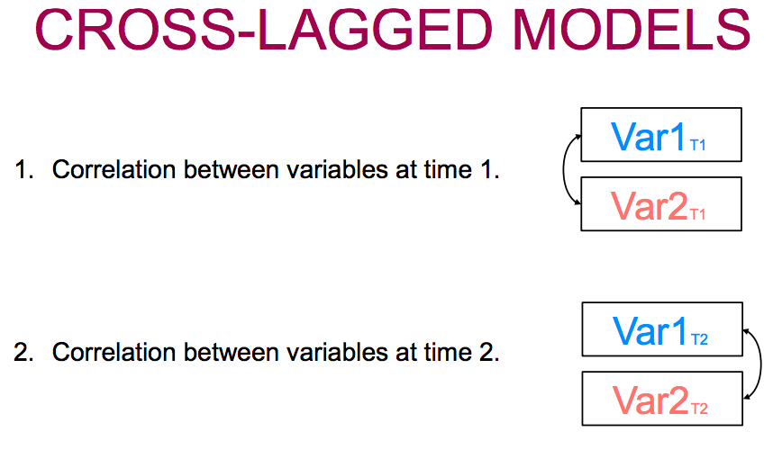
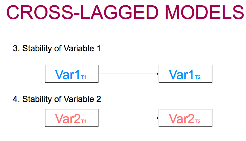
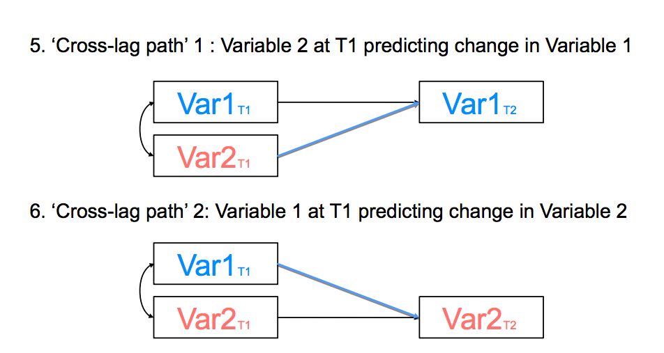
There are 6 parameters to a two-wave crosslagged model.

1. Correlation between variables at time 1.

2. Correlation between variables at time 2. Var1T2

3. Stability of Variable 1

4. Stability of Variable 2

5. ‘Cross-lag path’ 1 : Variable 2 at T1 predicting change in Variable 1

6. ‘Cross-lag path’ 2: Variable 1 at T1 predicting change in Variable 2

ASSUMPTIONS OF LONGITUDINAL ANALYSIS

Inter-individual stability

These techniques examine stability and change in the sample over time.

Thus, it is assumed that there are no systematic differences in the stability and change between the participants.

This assumption is violated when one group of participants changes faster or slower relative to the other participants.

Consistent Measurement

It is assumed that the measurement is the same when using repeated measures (i.e. the same measure over two or more time periods).

In practical terms, this means that the items administered to participants need to be exactly the same across time periods.

In conceptual terms, participants need to read and interpret the questions in exactly the same way across time periods.

Synchronicity

It is assumed that the administration of questionnaire occurs with the same interval between time periods for all participants.

CONSIDERATIONS OF LONGITUDINAL ANALYSIS

Timeframe

• In order to find a longitudinal effect, the length of time between measurements need to be considered.

The timeframe may be too short for a variable to impact another, and so you won’t find an effect.

The timeframe may be too long and the impact of one variable on the other may have dissipated

Other variables (third variable effect)

It is important to ensure that important variables are not omitted.

This idea is related to a causal process or pathway.

For this reason, it is easier to say that a variable at time 1 influences or impacts something, rather than causing it.

Summary

The cross-lagged design is the gold standard of panel designs

It overcomes the limitations of the previous designs by testing for uni-directional and bi-directional relationships The 2-wave cross-lagged design has 6 parameters:

Cross-sectional associations between the variables at T1 & T2

The association over the time for each variable (stability/change)

The cross-lag paths for each variable at T1 predicting the other at T2

The longitudinal design have several assumptions including: inter-individual stability; consistent measurement; synchronicity

Other considerations include the length of the timeframe and potential other variables

Página 14

Week 12

The Replication Crisis

WHAT IS THE REPLICATION CRISIS?

The Replication Crisis in Psychology

Originated in the early 2010s

Finding that research studies could not be replicated

Independent researchers following the same procedures as original studies could not find comparable results

Led to the ongoing questioning of established phenomenon and recommendations for the scrutiny of research practices

What triggered the Replication Crisis?

Bem (2011) Precognition - an ability to “feel the future”

Nine experiments:

Retroactive facilitation of recall

Recall of information (words) was better when never initially exposed to the information

This is contrary to everything we know about remembering information (e.g., rehearsal)

Encouraged other researchers to replicate the findings

Three replication attempts were made by other researchers

Not one could replicate the results

Coined the terms:

Questionable research practices (QRP’s)

p-hacking

Hacking data until you get the required p value to publish a study

E.g., Used a real dataset to demonstrate that listening to the Beatles song When I’m 64 made people younger

Obviously this is not possible (make people younger)

By using computer simulations to demonstrate that various decisions about data analyses made the results significant

Diederik Stapel • Nov 2011 • Fabricated data • 50 papers retracted

THE REPRODUCIBILITY PROJECT

“Reproducibility”

Reproducing results when reanalysing the original data

“Replication”

Replicating results from new data sets

Started in November 2011 by developing a protocol for selection and conduct of the replications.

270 contributing authors !

Looked at effect size as well as significance

Converted the results to correlations (recall this in the Person-Situation Debate?)

Only 36% of the replications were "successful" (i.e., produced p values < .05)

Summary of findings

Only 36% of the replications were "successful" (i.e., produced p values < .05).

The average effect size of the replications was around half that of the original studies.

Weaker, more surprising findings were less likely to replicate.

Social psychology findings were less than half as likely to replicate as findings in cognitive psychology.

REPLICATION CRISIS

A growing log of phenomenon that do not replicate

Stereotype threat

Ego-depletion

Power poses

Priming

The Stanford Prison experiment (this week’s podcast)

Why does this happen

Questionable Research Practices (QRP)

p-hacking

Removing participants

Not reporting all experimental conditions

HARKING

Hypotheses After the Results are Known

Publication bias

Small samples (in original studies)

Open Science

CHANGES TO THE FIELD

Led to a greater emphasis on Open Science:

Pre-registration

Open access to (deidentified) data

Open access to materials

Open access to results

PRE-REGISTRATION

Preregistration (aka unreviewed preregistration)

Researcher creates a detailed description of their plans for their study and records this is a timestamped, unedited archive

The plan can be shared with others

Registered Reports (aka reviewed preregistration)

Research submits a detailed proposal of their planned study to a journal for a review of the planned methods and analysis

Similar to Preregistration but addresses publication bias (results are published regardless of the outcome)

Some journals require this

Registered Replication Reports (RRR)

Similar to Registered Reports but focus on direct replication of original findings

Numerous labs follow the same preregistered plan and the results are reported collectively

E.g., ManyLab project

Open access to all data

All original data (deidentified) collected is placed in an online archive

Some funding agencies and journals make this a requirement

Materials used to inform the methodology is provided

Measures Ethics approvals

OPEN PRACTICES

Open access to decisions with “cleaning” data

Open access to analyses performed

Open access to preprints

Version of a journal article before it is typeset by the journal

Access to preprints

Sharing of code

And more

OPEN SCIENCE BACKLASH

A lot of backlash from established researchers (who typically benefit from flashy novel findings) as to this move to Open Science and the replication initiatives

“Tone”

"shameless little bullies”

"Methodological terrorists”