
Flashcards
BA Module 1
Flashcards do conjunto (41)
- 1Some people are naturally more comfortable working with numbers than others. For most of us, visual representations of data make it easier to identify trends and patterns that can help us make better decisions. This is especially true for large data sets; the more data we have, the harder it typically is to distinguish trends and patterns based solely on reviewing the data set.Data visualizations are all around us. The nutritional information on a cereal box offers a standardized format that helps us understand how a single bowl of cereal fits into the context of our overall daily food intake. The dashboard on your car is a visual representation of complex data about a car’s performance—such as its speed, fuel and oil levels, and whether or not its headlights are on. The dashboard has been carefully designed to help us understand how the car is operating with only a quick glance.
- 2In addition to graphing data, we can group data into categories that make it easier to perform analyses within a category or across multiple categories. The groupings we choose are often influenced by the question we are asking or the problem we want to solve. An income statement, also known as a profit and loss (P&L) statement, is a good example of a way to arrange financial data to make it easier to understand. Accountants separate data into categories such as income and expenses so companies can analyze their performance.Statements with financial data can look intimidating at first, but you’ll become comfortable using them more quickly than you might think. Over time, most managers become as adept at understanding a balance sheet or P&L as a driver is at monitoring a car’s performance by taking a quick glance at the dashboard.
- 3What is a histogram and what is it's use?One of the most useful and commonly used graphical representations of data is a histogram. A histogram displays the frequency, or number, of data points (often called observations) that fall within specified bins.
- 4Histograms allow us to discern _______ in a data set and are easy to construct using Excel.Trends or patterns
- 5How are the axis of a histogram defined in Excel?On the horizontal axis, we display a series of single values, each of which represents a bin, or range of possible values. On the vertical axis, we display the frequency of the observations in each bin. With a small data set, we can count and assign data points to bins as we just did, but with large data sets, this approach would be extremely tedious. This is where programs like Excel are helpful!
- 6What is skewness?The histogram you just created is skewed, meaning that it has a tail that extends out to one side. The tail is the part of a graph that appears long or “flattens”, and has bins with lower frequencies. Skewness measures the degree of a graph’s asymmetry. If the right tail is longer, we say the distribution is skewed to the right or “right-tailed.” Likewise, if the left tail is longer, we say the distribution is skewed to the left or “left-tailed.” The oil consumption data set is skewed to the right.
- 7Data points that fall far from the rest of the data are called _______Outliers
- 8What questions to ask when we see an outlier?When we see an outlier, we should investigate why it exists. Is it just an unusual but valid data point? Is it a data entry error? Was it collected in a different manner or at a different time than the rest of the data?
- 9What are the approaches to take when we see an outlier?Typically, we take one of three approaches when we see an outlier:
* leave it as is
* change it to a corrected value,
* or, very rarely, remove it from the data set. - 10Technical definition of an outlierTechnically, a data point is considered an outlier if it is more than a specified distance below the lower quartile or above the upper quartile of a data set. Let’s start with a couple of definitions. The lower quartile, Q1, is the 25th percentile—by definition, 25% of all observations fall below Q1. The upper quartile, Q3, is the 75th percentile—75% of all observations fall below Q3. The interquartile range (IQR) is the difference between the upper and lower quartiles, that is, IQR=Q3–Q1. We then multiply the IQR by 1.5 to find the appropriate range, computing 1.5(IQR)=1.5(Q3–Q1). A data point is an outlier if it is less than Q1–1.5(IQR) or greater than Q3+1.5(IQR)
- 11What should we do before gathering and analyzing data?Before gathering and analyzing data, we should always clearly articulate the question we wish to answer.
- 12____ measures the degree of a graph's asymmetry.Skewness measures the degree of a graph’s asymmetry.
- 13What are descriptive statistics?As we have seen, graphs are very useful for providing insight into a data set’s patterns, trends and outliers. However, sometimes we would like to describe the data in a more concise way, with just one or two numbers. We call such summary measures “descriptive statistics”—they provide a quick overview of a data set without showing every data point. We encounter these kinds of descriptive statistics every day: we talk about a baseball player’s performance by referring to his batting average; we measure stock market performance using the Dow Jones Industrial Average or the Nikkei Index; we summarize our academic performance using our grade point average.
- 14What is the "central tendency" of a data set?let’s determine the “central tendency” of a data set—an indication of where the “center” of the data set lies. We usually start by calculating the mean, the most common measurement of central tendency. The mean is the number people refer to when they talk about the “average” of a set of numbers.
- 15What are some methods of measuring central tendency?Mean: The mean is equal to the sum of all of the data points in a set, divided by n, the number of data points.
Median: The middle value of a data set. The same number of data points fall above and below the median. To find the median, first arrange the values in order of magnitude. If the total number of data points is odd, the median is the value that lies in the middle. If the total number is even, the median is the average of the two middle values.
Mode: The value that occurs most frequently in a data set. - 16What is the difference between mean of a sample and mean of a population?We represent the mean by x¯when we calculate the mean of a sample and by μ when we calculate the mean of a population. In the following definitions, n is the number of data points in a sample and N is the number of data points in a population.
- 17Briefly describe distribution with multiple modesThe mode is the value that occurs most frequently in a data set. If a data set has more than one value with the highest frequency, that data set has more than one mode. A distribution is called bimodal if it has two clearly defined peaks (two points with very high frequency). The two peaks may have equal frequency and hence be true modes, or one peak may be a mode and the other peak may simply have a very high (but not the highest) frequency. Distributions with multiple peaks are called multimodal.
- 18Mean, median, mode: which of these is not affected by outliers?Median and mode. Mean is affected by outliers
- 19What is the 25th percentile?Also known as the first quartile, the 25th percentile is the smallest value that is greater than or equal to 25% of the data points.
- 20What are percentiles used for?Percentiles are often used to categorize test scores. For example, someone who scored in the 95th percentile of a test scored equal to or higher than 95% of all people who took that test. We can also say that person scored in the top 5%.
- 21What formulas can be used to find the number corresponding to a percentile?Mean. Median, Mode. Mostly Median, eg to find the 95th percentile.
- 22Median is the same as 50% percentile. TRUE or FALSE?True. Median of a set of data is the 50th percentile. The percentile of the mean and mode cannot be determined without further information
- 23Apart from the mean, what other item is needed to summarize data numerically?As we've already learned, looking at the distribution of a data set is often very helpful. However, if we want to summarize the data numerically, we typically convey both the mean and a measure of variability.
- 24What is one way to measure variablility?One of the simplest measures of variability, or spread, is the range:
Range=Maximum value–Minimum value - 25Data sets that have the same min and max values will have the same range despite the distribution. What can we do to gain more insight into the spread of the distribution?To gain more insight into the spread of the distribution and how the data behave between the two extremes, we can calculate the variance. Rather than simply measuring the distance between the two extremes, the variance measures how far each point is from the mean.
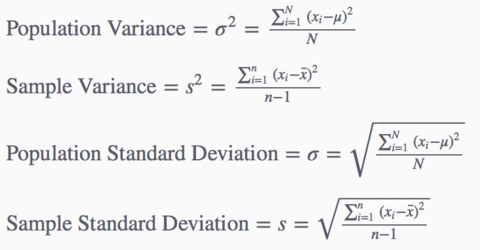
- 26What are the formulas for * Population Variance * Sample Variance * Population Standard Deviation * Sample Standard Deviation ?
- 27Calculating Measures of Variation for Populations and Samples. Talk about it briefly.When calculating σ2, the variance of a population, we divide by N, the size of the population. However, we rarely have information about an entire population, so we often estimate the variance and standard deviation based on a subset of the population, known as a sample (we will learn more about samples in the next module). When calculating s2, the sample variance, we divide by n–1, the sample size minus one. Dividing by n–1 corrects a bias that would occur if we divided by the sample size, n. For large samples, subtracting one is only a small adjustment, but for small samples, subtracting one can result in a much larger adjustment.
- 28Name a few measures of variability* Range
* Variance
* Standard deviation - 29What do small and large standard deviations indicate?A small standard deviation indicates
that the data points are close to the mean.
A large standard deviation indicates a broader spread.
Luckily, we can use Excel to calculate the variance in standard deviation.
We'll never have to do so by hand again. - 30What is: 1. Kurtosis 2. Skewness ?Excel’s actual descriptive statistics tool generates a few additional fields that are not seen in our version of the tool:
Kurtosis: a measure of the flatness or sharpness of a distribution. A flat distribution has low kurtosis; a very sharp distribution has high kurtosis.
Skewness: a measure of the degree of asymmetry of a distribution. - 31What is coefficient of variation and what is the formula?To compare variation in two data sets, we calculate a value called the coefficient of variation (CV). The coefficient of variation is the ratio of the standard deviation to the mean. The equation for the coefficient of variation is:
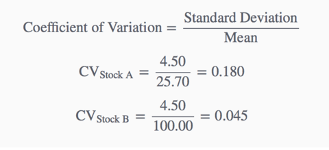
- 32When a question asks: which of the following data sets has the highest relative variation? What is it looking for?Coefficient of variation: Standard deviation / Mean
- 33While we use histograms to visualize a single variable's distribution, what do we use to visualize the relationship between 2 variables?We use histograms to help us visualize a single variable’s distribution. To visualize the relationship between two variables, we typically use a scatter plot. One variable is plotted on the horizontal axis (x-axis), and the other is plotted on the vertical axis (y-axis). Later in the course when we learn about regression analysis, we’ll see that the convention is to plot the so-called “dependent” variable on the vertical axis and the “independent” variable on horizontal axis.
- 34Apart from visualizing the relationship between 2 variables, what else are scatter plots good for?As we have seen, scatter plots are useful for visualizing the relationship between two variables. It is also helpful to have a measure that quantifies how strong the relationship is.
- 35Describe the correlation coefficient of a scatter plot?We will use the correlation coefficient to measure the strength of the linear relationship between two variables. The correlation coefficient measures the extent to which the data points on the scatter plot create a line, on a scale from -1 to +1. Move the slider to see how a scatter plot changes as the correlation changes.
- 36Is correlation coefficient enough to interpret a scatter plot?Even when the correlation coefficient is 0, a relationship between two variables might exist—just not a linear one. The relationship may appear more like a curve, for example, as shown below. Never rely solely on the correlation coefficient. Always consult a visual representation of the data such as a scatter plot to see patterns and gain other insights into the situation the data describe.
- 37Correlation indicates a linear relationship but does not indicate causality. Explain.The correlation of height and weight between the ten Red Sox players is quite high (0.8). However, a high correlation does not imply that one variable causes the other. Taller people may tend to weigh more, but gaining weight won’t make you taller! Correlation indicates a linear relationship, but it does not indicate causality.
Although there may be a relationship between two variables, we cannot conclude that one variable “causes” the other. This point is best summarized in the admonition, “correlation does not imply causation.” - 38What is a hidden variable?A hidden variable is a variable that is correlated with each of two variables (such as ice cream and snow shovel sales) that are not *fundamentally* related to each other. That is, there is no reason to think that a change in one variable will lead to a change in the other; in fact, the correlation between the two variables may seem surprising until the hidden variable is considered. Although there is no *direct* relationship between these two variables, they are mathematically correlated because each is correlated individually with a third “hidden” variable. Therefore, for a variable to act as a hidden variable, there must be three variables, all of which are mathematically correlated (either directly or indirectly).
- 39Give an example of a hidden variable.In the example above, season is correlated with ice cream sales (people are more likely to buy ice cream in the summer when the weather is hot). Season is also correlated with snow shovel sales (people are more likely to buy snow shovels in winter when the weather is cold and snow begins to fall). However, there is no direct connection between ice cream sales and snow shovel sales: ice cream sales don’t go up because no one is buying snow shovels, and people don’t purchase snow shovels because they are not buying ice cream. Nonetheless, the two variables are correlated because both ice cream sales and snow shovel sales are correlated with the same variable: season.
- 40What is a time series?Sometimes we are interested in the behavior of a single variable over time. In such cases, we can consider time as a second variable, which we typically show on the horizontal axis. Suppose that once we realize that the U.S. consumes more oil than any other country, we decide to look at U.S. oil consumption over the past eleven years to gain insight into the consumption trend. Create a scatter plot to help visualize the relationship.
- 41What is the difference between time series and cross sectional data?The data set we just used is called a time series—a data set in which one of the variables is time. Most of the data sets we have analyzed up until this point have been cross-sectional data. Let’s make sure we understand the difference between these two types of data sets.
Time Series vs. Cross-Sectional Data:
Time Series: Time series data contain data about a given subject in temporal order, measured at regular time intervals (e.g. minutes, months, or years). U.S. oil consumption from 2002 through 2012 is an example of a time series. Managers collect and analyze time series to identify trends and predict future outcomes.
Cross-Sectional: Cross-sectional data contain data that measure an attribute across multiple different subjects (e.g. people, organizations, countries) at a given moment in time or during a given time period. The average oil consumption of ten countries in 2012 is an example of cross-sectional data. Managers use cross-sectional data to compare metrics across multiple groups.
Informações
- Descrição
- Business/Economics FlashCards sobre BA Module 1, criado por Sola So em 30-07-2016.
- Criado por
- Sola So
- Visualizações
- 2
- Avaliação