Unit 12 Algorithms

Unit 12 Algorithms

1. T1 - Analysis & Design of algorithms

   • Problems solved by algorithms
     • A good algorithm
       • has clear and precisely stated steps that product the correct output for any set of valid inputs
       • Should allow for invalid inputs
       • Must always terminate at some point
       • Should perform the task efficiently, in as few steps as possible
       • should be designed in such a way that other people will be able to understand it and modify it if necessary
   • Execution time VS problem size
     • For most problems, the larger the size of the problem or amount of data, the longer the execution time
   • Linear function
     • A linear function takes the form f(n) = an + b where a and b are constants
     • F(n) = 3n, f(n) = n + 5 are examples of linear functions
     • F(1) is a constant function - no matter how large n gets, f(1) stays the same size. F(2), f(3) and f(100) are all constant functions.
     • The order of magnitude for a linear function is written as O(n)
   • Quadratic function
     • A quadratic function takes the form f(n) = an^2 + bn + c where a, b and c are constants.
     • As n becomes large, the n^2 terms increases very much faster than either of the other terms
     • The order of magnitude of a quadratic function is written as O(n^2)
     • The dominant term is the one used when comparing algorithms, so the bn and c terms are not considered
   • Logarithmic functions
     • A logarithmic function takes the form f(n) = alog2n. the logarithm of a number is the power to which the base must be raised to make it equal to a number
     • 8 = 2^3, log2,8 = 3, this is an example of a logarithmic function
     • F(n) increases very slowly in relation to n. The order of magnitude of a logarithmic function is written as O(log n)
     • Logarithmic function
       • "Divide and conquer" algorithms work by halving the size of the problem at each pass. A binary tree search algorithm is a good example of this.
       • For a balanced tree of 1024 (2^10) items, only20 items need to be examined
       • Time complexity increases very slowly as the problem size increases. It is logarithmic, that is, O(log n).
   • Big-O notation
     • Big-O notation is a measure of the time complexity of an algorithm. It is a useful approximation of the time taken to execute an algorithm for a given number of items in a data set.
     • An algorithm of time complexity O(n) increases linearly. 10,000 items will take approximately twice as long as 5000 items to process
     • There is no such thing as, for example, O(2n+1). Only the dominant term counts, so it is O(n)
   • Permutations
     • A permutation of n items is the number of ways the n items can be arranged.
     • Repetition allowed; for example, a combination lock with 4 digits 0 to 9
     • No repetition allowed; for example, you have 4 different coloured balls in a bag, and you draw them out one at a time

2. T2 - Searching Algorithms

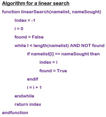
   • Linear Search
     • if the data is in a random order, the only systematic way to find something would be a linear search
       • Algorithm for a linear search
     • Big-O for linear search
       • There are 2 statements in the loop and 3 at the start. 2n + 3 in worst case. The time complexity is O(n)
   • Binary search
     • The binary search is a very efficient way of searching a sorted list.
     • Examine the middle item in the list
       • If this is the one you are searching for, return the index
         • Eliminate half the list, depending on whether the item being sought is greater than or less than the middle item
           • Repeat until the item is found or is proved top be not in the list
   • Divide & Conquer
     • In a binary search, the size of the list is approximately halved each item an item is examined
     • In a list of 2^n items, the maximum number of items you will need to look at will be n + 1

3. T3 - Bubble & Insertion Sort

   • Choosing a sort algorithm
     • If there only a small number of items to sort, a bubble sort may be perfectly adequate
     • Some sort of algorithms take a lot of memory and that may be a problem with a large dataset
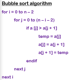
   • Bubble sort
     • A bubble sort is a useful sort when there are only a small number of items to be sorted
     • To sort an array of n items, n-1 passes are made through the array, with each item being compared with the adjacent item and swapped if necessary
     • Big-O for a bubble sort
       • The three statements in the inner loop are performed n(n-1 + n-2 + n-3 + ...... + 1)
         • This is approximately 3 x 1/2 n^2 statements. Ignoring the constant, the time complexity is O(n^2)
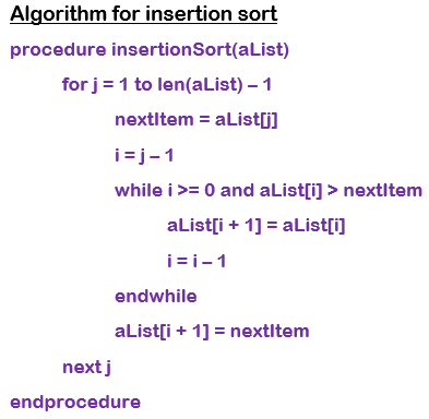
   • Insertion sort
     • The insertion sort is an efficient algorithm for sorting a small number of elements. It works in the same way you might sort a deck of playing cards
     • Start with all cards face down. Pick up each card in turn and insert it into the correct place in the deck.
     • Time complexity of insertion sort
       • The insertion sort algorithm has 2 nested loops, the outer loop is performed n-1 times, the inner loop, which moves the items along to make room for the current item, is performed a maximum of n-1 times, the Big-O time complexity is O(n^2)

4. T4 - Merge & Quick sort

   • Merge sort
     • This is much more efficient than the bubble sort
     • Big-O for the merge sort
       • This is another example of a 'divide and conquer' algorithm which halves the size of each list to be merged
       • First the list is split into halves, log2n times. Each of these log2n splits requires n operations to merge the data into a single list
       • So the time complexity is O(n log2n)
   • Quick sort
     • This is another 'Divide and Conquer' algorithm. It is much faster than any of the other sorts.
     • The algorithm works by finding a split point, which divides the lists into two sub-lists, one containing items less than the value at the split point, and the right half containing items greater than the value at the split point

5. T5 - Graph traversal algorithms

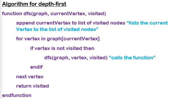
   • Depth-first traversal
     • With depth-first, you go as far as you can down a path before backtracking and going down the next path
     • The algorithm uses a stack to keep track of the last node visited, and a list to hold the names of nodes that have been visited
     • Applications of a depth-first traversal
       • Job scheduling, where some jobs have to be completed before others can begin

Bilder und Dateien der Mindmap