week 3

Page 1

classification problems:

binary : yes/no; true/false ; malignant/benign tumor; spam/no spam

y = {0 , 1}

multiclass : y = { 0 , 1 ,2 ,3 }

using linear regression for classification:

you cannot use lnear regression for classifcation problems as 'y' in linear regression can <0 or >0;

in logistic regression : 0 <= h-theta(x) <= 1

Page 2

Logistic regression:

linear regression hypthesis :h-theta(x) = thetaTranspose * X

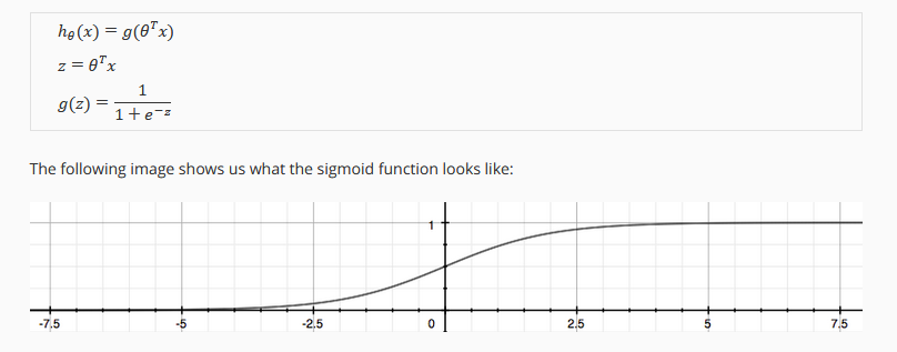
Logsitic regression : hypothesis : h-theta(x) = g (theta-transpose * X)

where g(z) = 1/( 1 + e^-z)

so logistic regression function : h-theta(x) = 1/(1 + e^ (-thetaTanspose * X))

so objective in logistic regression : find theta such that 'y' represents the sigmoid fucntion or logistic function for the given

ex., x = [ x0 = [1

x1] tumor size] ;

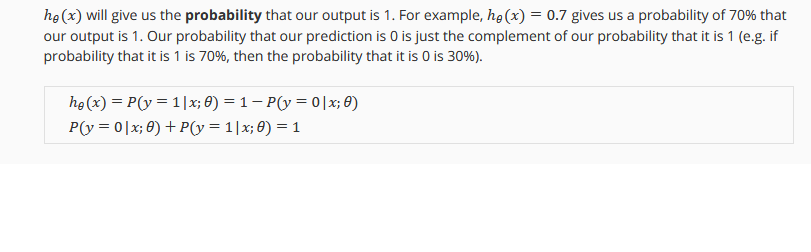
if h-theta(x) = .7 ;

probability that the tumor being malign is 70%;

ie., h-theta(x) = P(y=1 |X ;theta) : probability that y=1 , given x, parametrized by theta;

h-theta(x) gives the probability that y=1;

Page 3

logistic regression:

h-theta(x) = g(theta-T *X)

g(Z) > = .5 , Z >=0

two variable regression:

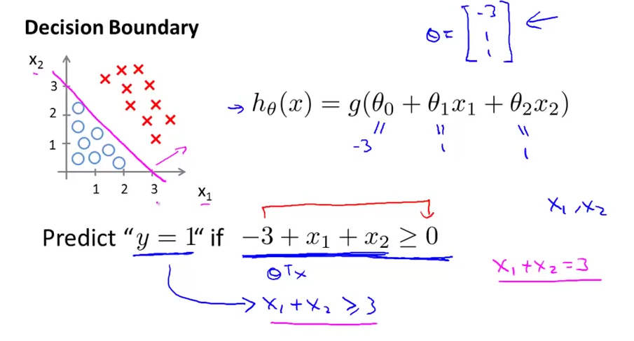
h-theta(x) = g( theta-0 + theta1-x1 + theta2-x2)

theta-0 + theta1-x1 + theta2-x2 > =0

limiting condition :say

theta-0 =-3;

theta -1 = 1

theta-2 = 1

predict y = 1 , when , x1 + x2 >= 3

x1 + x2 = 3 is the decision boundary (straight line in this case);

that seperates : y =1 & y= 0;

Page 4

Decision Boundary:

In order to get our discrete 0 or 1 classification, we can translate the output of the hypothesis function as follows:

hθ(x)≥0.5→y=1

hθ(x)<0.5→y=0

The way our logistic function g behaves is that when its input is greater than or equal to zero, its output is greater than or equal to 0.5:

g(z)≥0.5 whenz≥0

Remember.

z=0,e0=1⇒g(z)=1/2

z→∞,e−∞→0⇒g(z)=1

z→−∞,e∞→∞⇒g(z)=0

So if our input to g is θTX, then that means:

hθ(x)=g(θTx) ≥0.5 when θTx ≥ 0

From these statements we can now say:

θTx ≥ 0 ⇒ y=1

θTx < 0 ⇒ y=0

The decision boundary is the line that separates the area where y = 0 and where y = 1. It is created by our hypothesis function.

Example:

θ=5−10y=1

if 5+(−1)x1+0x2≥0

5−x1≥0

−x1≥−5

x1≤5

In this case, our decision boundary is a straight vertical line placed on the graph where x1=5, and everything to the left of that denotes y = 1, while everything to the right denotes y = 0.

Again, the input to the sigmoid function g(z) (e.g. θTX) doesn't need to be linear, and could be a function that describes a circle (e.g. z=θ0+θ1x1^2+θ2x2^2) or any shape to fit our data.

Page 5

cost function for logistic regression:

J(theta) = 1/m *(sigm1 1 ->m) (Cost(h-theta(x), y)

cost ( h-theta(x) , y) = { -log(h-theta(x) , if y = 1;

-log(1 - h-theta(x) , if y = 0; }

Page 6

problem of overfitting:

fit explains e training set data very well...not generic enough to explain the test data

how to deal with overfitting? :

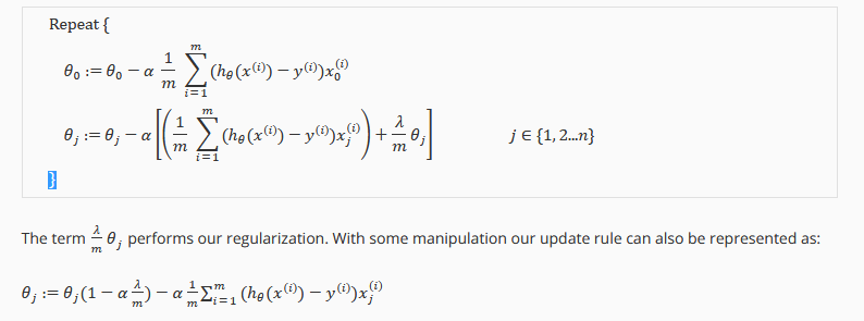
introduce a regularization parameter lambda :

that will will assign small values to higher oreder thetas (theta-3, theta-4) to minimize impact of overfitting

Page 7

regularized logistic regression:

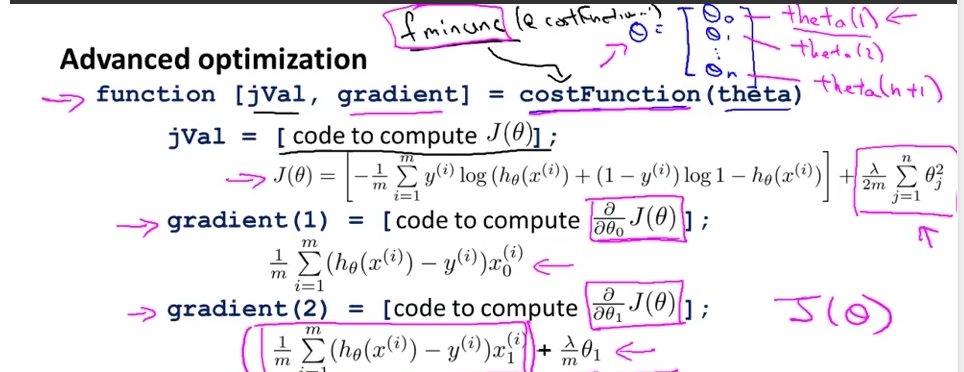
compute cost function : J(Theta)

compute the gradients : gradient 1 , gradient 2 ....gradient (n+1)