Flashcards

Stats

Skye Stuart English 187 cards

Cards in this deck (187)

1How do you decide how many replicates needed in a sample?✔Conduct a formal power analysis
2How is power increased?INCREASE Sample size – larger = greater confidence in where the pop mean is going to be
INCREASE Effect size (difference between the groups). Big = easier to detect
INCREASE significance level to P<0.01 – careful! This will also increase type 1 error rate
DECREASE Random variation (variability in data)
3How and why do you conduct a formal power analysis?To know how many replicates needed in a sample:
Power –probability of detecting a diff if one is really there to be detected
Power = 1- type II error rate (β)
e.g. Power of 80% = type II error rate of 20%
4Shapiro WilkTest for normality
• P<0.05 = data is not normally distributed
• P> 0.05 = data is normally distributed
5What to do to prevent problems with multiple comparisons tests?• FDR – false discovery rate
• Controls for a percentage of false positives
6Cooks distanceProvides a measure of the overall influence of a data point on the overall model,
>1 PROBLEM
- More useful than leverage alone
- Combines distance and leverage as one number
More common rule problem if Cooks distance > 4/n – cut off for ANOVA and linear regression
7Residualdistance from regression line
* will affect the effect of that data point on the quality and robustness of the model
8Leveragehorizontal distance from mean of the predictor/ centre line of gravity (dotted line)
* will affect the effect of that data point on the quality and robustness of the model
9Independent variableX AXIS
What you are manipulating/ controlling
10Dependent variableY AXIS
What you are measuring
- observed effect
- Interested in predicting
11Nominal variableVariables that have two or more categories, but which do not have an intrinsic order
e.g. "type of property" is a nominal variable with 4 categories called houses, condos, co-ops and bungalows
12Dichotomous variablesNominal variables which have only two categories or levels
e.g. Gender - male or female
13Ordinal variablesVariables that have two or more categories just like nominal variables only the categories can also be ordered or ranked
e.g. Economic status, with three categories (low, medium and high)
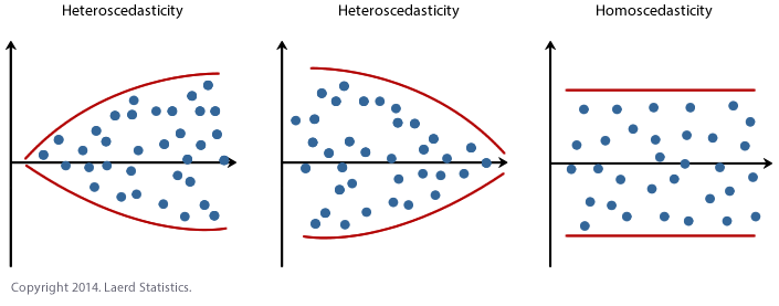
Cannot place a "value" to them
14What does homo/heteroscedasticity look like?
15Equation for determining CI for proportions from SEStandard error (SE) of the proportion = -->
CI for the proportion = +-(1.96 x SE)
P = proportion
16Example using CI SE of proportions: 64 women with bleeding disorder, 27 reported bleeding gums once a week. What is our CI for the prevalence of bleeding gums in pop of women with bleeding disorder?P = 27/64 = 0.422
= SqR (0.422 x0.578/64) = 0.0617 (6.17%)
CI for the proportion = +/- (1.96xSE) = +/- (1.96x0.0617) = 0.121
Proportion is 42.2% (30.1% to 54.3%)
* times everything by 100
17Standard error of mean + EQUATIONStandard deviation of a sampling distribution.
Measures accuracy with which the sample represents a population
o If large, a lot of variability between means of diff sample so samples might not be representative of population
o SEM – no overlap can or can’t mean significance
BETTER TO USE 95% CI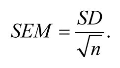
18VarianceThe average of the squared differences from the Mean
19Standard deviationmeasure of how spread out numbers are
- square root of variance
20Equation for determining CI when question has mean and SDX = mean
1.96 = Z score
s = SD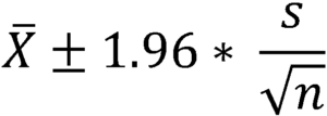
21What is the coefficient of determination (r2)? + EQUATIONProportion of variability explained by the predictor
• Amount of variation explained by model
Fit of regression - how well the model explains the data
r2= SSM/SST
22What does the F ratio describe? Equation for F ratio• How well data fits to straight-line model.
• HIGHER f ratio = LOWER p value = MORE significant = closer data points are to straight line
• Larger the F ratio = more variability can be explained by that line
F ratio = MSM / MSR
23Variance Inflation Factor• Detects multi-collinearity in regression analysis
• Estimates how much r2 increases due to multicollinearity
VIF >10 problematic (substantial degree of collinearity)
Average VIF> 1 problematic
• The more VIF increases, the less reliable regression results are
24Welch's correction or Browne-ForsytheNonparametric equivalent of unpaired t-test and ANOVA if only homogeneity of variance violated
*works to adjust the residual degrees of freedom
25Levene's Test• Parametric test for homogeneity of variance (variances are equal)
• P>0.05 to pass Levene’s test
- If doesn’t pass use P values that don’t assume variance
- If it doesn’t pass – can’t use one-way ANVOA as it assumes variance across the groups
26Familywise error rateprobability that we will make at least one Type I error in a set (family) of comparisons
27P = 0.05there's a 5% chance of getting your observed result, if the null hypothesis were true. It does not mean that there's a 5% chance that the null hypothesis is true.
28Advantages of planned contrasts• If product of contrasts = 0 – contrasts are orthogonal and statistically independent and can trust results of contrasts without performing multiple comparisons
• Don’t need to correct for number of tests performed
• Power of tests are higher than post hoc multiple comparisons
• More likely to detect a difference than a multiple comparison test which compares all groups against all other groups
29How to interpret interaction plots• Horizontal lines indicate no significant main effect of dose.
• Overlapping lines indicate no significant main effect of sex.
• Parallel lines indicate no significant interaction.
• BELOW lines are parallel so there is no significant interaction, but there are significant main effects of both dose and sex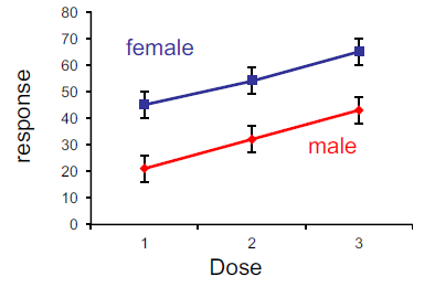
30What is an interaction?Interaction observed between two factors whenever the simple effects of one change as the levels of the other factor are changed
• Interaction when lines are not parallel
• Requires 3 factors; two independent and one dependent
31What is a main effect?the overall effect for one factor
32EC5050% of response
33Equation for non-linear regression
34Factorscan be manipulated or are of interest experimentally
35Factorial ANOVAAnalysing more than one factor at the same time
36Residual variabilityvariability in these measures within an individual
37Log transformationMakes big numbers small
Use if:
- Data are highly skewed (positive or negative)
- Data contains large range of values for independent variable (over several orders of magnitude)
38Z valuescalculates standardised scores
*can judge how far a value is from centre compared to spread of the data
39Confidence IntervalsA range to estimate an unknown population parameter with a given confidence level
• Population mean will fall within this range in 95% of samples
- CI can’t overlap with 0 or 100 = no significance
40Confidence leveldegree of confidence e.g. 95% sure
41Confidence limitthe upper and lower values of the interval e.g. upper = 95, lower = 15
42What is the SE if the CI is 68%?68% CI = ± 1.0 x standard error
68% of total area under the curve is within 1 SD of the mean
43What is the SE if the CI is 95%?95% CI = ± 1.98 x standard error
95% of total area under the curve is within 2 SD of the mean
- Approx. 95% the mean of normally distributed sample will lie within +- 1.96 SD from the mean
44What is the SE if the CI is 99%?99% CI = ± 2.6 x standard error
99% of total area under the curve is within 2.6 SD of the mean
45What is the SE if the CI is 99.9%?99.9% CI = ± 3.3 x standard error
99.9% of total area under the curve is within 3.3 SD of the mean
46Non-parametric alternative to Paired T-testWilcoxon signed-rank test
47Non-parametric alternative to Unpaired T-testMann-Whitney U test
48Non-parametric alternative to One-way ANOVAKruskal-Wallis Test
49Example of single sample t-testWhether performance of two groups of students is significant diff from historic average of 59.1
- H0= mean mark is equal to 59.1
- HA = mean mark is not equal to 59.1
50Single sample t-test- Test value = average comparison value (e.g. average mean from previous years)
- Null hypothesis has the population mean equal to a specified value
51Two sample t-test• Compares two samples of continuous data to test for significant differences
• Testing the null hypothesis, whether the difference between the sample means is equal to zero
• Homogeneity of variances
52Example of Two sample t-test- H0 = Difference between sample means = zero (i.e. sample means don’t differ significantly)
- HA = Difference between sample means ≠ zero (i.e., sample means are significantly diff)
53Paired vs unpaired t-testThe paired t-test reduces inter-subject variability and is more powerful than the unpaired t-test
54Wilcoxon Signed-Rank testNon-parametric test for two sample comparisons with PAIRED data
- Compares sample medians to see if the diff in medians = 0
55When is Wilcoxon Signed-Rank test used?1) Sample variances are substantially diff
2) If sample size is too small (<30)
3) In the case of ordinal, interval or ranked data
56How to quote Wilcoxon SR data?• T significance statistic in Wilcoxon SR
• Absolute no. of pairs in brackets not DF
57Mann-Whitney-U test• Non parametric test to compare two UNPAIRED samples integer or ordinal data
- Less influenced by skewness, non-normality and outliers because not based on mean
Quote U = Mann-Whitney-U value
58McNemar's test≥2 groups to test that 2 proportions are EQUAL and the data is PAIRED
▪ Same as paired t-test for nominal data
59Chi-squared test≥2 groups to test that 2 proportions are EQUAL and the data is UNPAIRED
o If expected values are >5 in 80% of cells or more
• Determine a significant difference between expected frequencies and observed frequencies
• Greater the diff between the expected and actual distribution, the larger the chi-square statistic
SYMMETRICAL
60Fisher's exact test≥2 groups to test that 2 proportions are EQUAL and the data is UNPAIRED
o If expected values are ≤5 in 20% of cells or more
• Used when chi-squared assumption is violated
• Calculates EXACT probability of that distribution of data or more extreme
NOT symmetrical
61Expected cell frequency equationIf E < 5 the test becomes inaccurate as Type I error increases - use Fisher’s Exact test which calculates an exact value for P
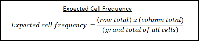
62Example of chi-squared testE.g. is there an ASSOCIATION between treatment and patient outcome?
Drug/Placebo and Effect/No effect to create a 2x2 contingency table
63What is most biologically important?Size of effect NOT statistical significance
Best to use P values but give effect sizes and CI intervals
64What is Bias?Anything that leads to systematic errors, not only the preconceived notions of the experimenter. Caused by any factor that will consistently alter results. Doesn't contribute to scatter as it will increase or decrease all values. Statistical calculations can't detect or correct bias (unless you do more experiments)
65What is confounding?When results can be explained in more than one way. The confounding variable is associated with the desired outcome and treatment group/risk factor. Confounding variables complicates analysis
➢ A confounding variable is an extra variable you didn’t account for
66How to quote Chi-square statistic?Quote is Pearson Chi-square value
67Crammer's V statisticStandard effect sizes from correlation data
Varies between 0 (no association) and 1 (full association) between the variables
• 0.1 – 0.3 = small effect size
• 0.3 – 0.5 = medium effect size
• > 0.5 = large effect size
68Correlation• Measures degree of ASSOCIATION between two paired sets of data/ variable
• NOT causality
• Only state they’re ASSOCIATED, as one increases, the other variable increases
• Correlation analysis doesn’t show anything about the relationship between variables
69Bivariate correlationRunning Pearson and Spearman's correlation at the same time
70Pearson correlation• Parametric test for straight linear associations between two continuous variables
• Measures the strength and direction of LINEAR ASSOCIATION that exists between two continuous variables
DF = N-2 (compares 2 variables)
71Assumptions of Pearson Correlation1. Continuous quantitative data on an interval or ratio scale
2. Linear relationship between x and y
3. X and y are measured independently
4. X and Y values sampled from a bivariately normally distributed population
5. NO significant outliers – r sensitive to outliers
6. Homoscedasticity of data
72Pearson correlation coefficient (r)Measures how close data points are to the line.
Can be a very shallow line but if data points are all on a straight line = 1.
• r provides no info about the slope
• r statistic gives most info not p
• r statistic gives you size of association i.e. effect size
• Closer to 1 = highly correlated
73What does a Pearson coefficient = 1 say about the linear relationship?Perfect straight line with positive slope
Perfect positive linear relationship
74What does a Pearson coefficient = 0 say about the linear relationship?No linear relationship between x and y
• Perfectly horizontal or vertical data
75What does a Pearson coefficient = -1 say about the linear relationship?Perfect straight line with negative slope
• Perfect negative linear relationship
76What does a Pearson coefficient +/-0.1 to 0.3 say about the strength of the association?Small correlation
77What does a Pearson coefficient +/-0.3 to 0.5 say about the strength of the association?Medium/moderate correlation
78What does a Pearson coefficient +/-0.5 to 1.0 say about the strength of the association?Large/strong correlation
79Coefficient of determination (r2)• Proportion of total variances shared by two variables
- Shows total variation in the data
• Amount of variation (%) explained by the correlation model
• Determines how strong the association is between two variables
80Spearman's rank correlation• NON-PARAMETRIC
• Measures the strength and direction of MONOTONIC ASSOCIATION between two independently ranked variables (not necessarily linear)
• Spearman’s rank is less sensitive than Pearson to outliers
• DF = N-2 (comparing 2 variables)
81Spearman rho value (rs)• Value between -1 to +1
• Closer to 1 = highly correlated
• Can’t square rs Can’t comment on proportion of variability accounted for by this association
82Cohen's dStandardised effect size for a difference between means
• Effect of each group compared to the other
• Pearson’s coefficient (r) also measures effect size
83Equation for Cohen's dd = difference in means/ SD of pooled means
84What formula links the correlation coefficient (r) with Cohen's d?r2 = d2/ (4+d2)
85How can the correlation coefficient (r) be calculated for a t-test?
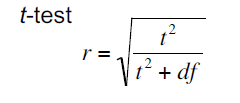
86How can the correlation coefficient (r) be calculated for ANOVA?ANOVA:
r2 = sum of squares group / sum of squares total
87How do the r and d values describe effect sizes?SMALL = r (0.1) = d (0.2)
MEDIUM = r (0.3) = d (0.5)
LARGE = r (0.5) = d (0.8)
A statistically significant measure with small effect size or greater indicates a meaningful difference
88Regression analysisChange in the X variable leads to a change in the Y
• Determines how well the data fits a theoretical model (line)
• Able to obtain a predictive relationship
89Assumptions for Regression1. Linear relationship between x and y
2. X and y are asymmetrical – X predicts Y
3. Data points (residuals) are independent (Durbin Watson)
4. For each X value the Y value is sampled from an approx. normally distributed population
o Normally distributed around the regression line with a mean of zero
5. HOMOSCEDASTICITY (constant variance)
• Doesn’t have a non-parametric equivalent – if assumptions aren’t met can’t perform regression
90Simple linear regression• Single independent variable (x-axis variable)
• Fit a line or model to describe the relationship it has with a single dependent (y-axis) variable
• Calculates the best straight line through the data – the line that minimises the sum of squares of the Y residuals (SSR)
91What are the sources of variability?• Distance between data point and the model (black line) = residuals so calculate SSR
• Distance between model and null hypothesis (blue) = SSM
• Total variability in data is given by the distances between each data point and the null hypothesis mean y line (blue)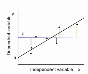
92Sum of squares equationSST = SSM +SSR
o SSM= sum of squares for the fitted regression line
o SST= total amount of variability within the data
o SSR – Sum of squares residual error. Distances between individual data points and the line that we’ve fitted – random unexplained variability
93What are the generalised hypotheses for simple linear regression?• H0: slope b = 0
• H1 : slope b ≠ 0
94Calculating r2 from regression analysisr2= SSM/SST
95Equation for Means squareMean square = Sum of Squares/ DF
• dfr = the model degrees of freedom (dfr = k - 1)
• dfe = the error degrees of freedom (dfe = n - k - 1)
• k = the total number of groups (levels of the independent variable)
• dfT = the total degrees of freedom (n - 1)
96Rules of regression models for identifying potential outliers1. Standardised residuals (measured in SD units above mean) >3 worth checking as an outlier
2. >5% of Residuals are >2 indicates model is poor fit
3. COOKs distance >1 is a cause of concern- should remove data point.
4. Worth investigating if Leverage Value >2 (k+1)/n
5. Standardised DFFIT and Standardised DFBeta >±1 shows substantial influence on the model
• Can’t just identify influential data points by standardised residuals – can have a low SR but strongly influence model
97Standardised DFFit and standardised DFBeta• Found under case summaries
• Standardised measures of how much the fit (how much does R^2 change)and slope of model would change if data point was removed
- Values >+-1 show substantial influence on model
**MOST USEFUL
98Assumptions of Multiple linear regression1. Dependent variables should be quantitative and continuous
2. Independent/ predictor variable should be quantitative or categorical, with only two categories
3. Linear relationship with non-zero variance (requires some variance)
4. HOMOSCEDASTICITY (residuals plot)
5. Independence of residuals
6. Random normally distributed residuals
7. Avoid ENTANGLEMENT- independent variables should not derive dependent variable e.g. Weight and BMI
8. No MULTICOLLINEARITY
9. Sample size should be at least 10X number of predictors tested
99How to check for multicollinearity?Inspection of correlation coefficients and Tolerance/VIF values
VIF>10 = high degree of collinearity
Average VIF> 1
Tolerance factor <0.1 problematic
100Durbin- Watson testIndependence of residuals
o Between 1.5 and 2.5
101Multiple linear regression• Fits data to a model that defines Y as a function of two or more variables, x1, x2
• Takes into account the relationship between x variables
102How is the residual calculated in multiple linear regression?Residual is the distance between each data point vertically down to that plane
Produces a plane not a line
103Equation for multiple linear regression• Extend the equation of straight line by adding another term
Y = b0 + b1x1 + b2x2 + …
Slope times predictor
b0= constant
104What is multicollinearity?When there’s correlation between predictors (independent variables) in a model
Can adversely affect regression results
105What is effect size?Measure of the size of the observed effect
- Difference between the groups regardless of sample size
- Measurement of the impact an independent variable has on a dependent variable
**Standardised effect size (d or r) accounts for variance
106Kruskal-Wallis test• Compares >2 samples with continuous data that DOESN’T satisfy parametric assumptions
• Rank-based approach for 3 or more unpaired samples
• Based on median rather than mean
** Only use when parametric assumptions are greatly violated
107Why are rank based tests more robust than parametric tests?Based on median rather than mean
Median is less influenced by outliers, skew and non-normality than the sample mean
108Assumptions for Kruskal -Wallis• Data are randomly sampled from populations
• Observations are independent
• Distributions are similar and homoscedastic
109Post Hoc testsUsed to perform multiple comparisons whilst controlling overall familywise type I error rate.
Used when there is no specific hypothesis to be tested.
• Compares each group with every other group to determine which group means are significantly diff
110Advantages of post hoc tests over multiple two sample t-tests?Post hoc tests compare each pair of means (like t-tests), but unlike t-tests, they correct the significance estimate to account for the multiple comparisons.
REDUCES POTENTIAL TYPE 1 ERROR
111Multiple comparison tests controls for what?Controls for getting a false positive finding at p<0.05 not just for a single test but across the family of tests you are performing
112Post hoc test assumptionsEqual variances assumed - assume homogeneity of variance
ANOVA assumptions must be met
113Tukey post hoc test• Compares means of every treatment to the means of every other treatment
• Best to use if sample sizes are equal,
• Good trade-off between type I and type II errors.
• Single step multiple comparison procedure and statistical test
• Used in ANOVA to create CI for all pairwise differences between factor level means,
114Dunnett's post hoc test• Best when interested in comparing all groups’ vs single control group (enables 1tailed tests)
• Performs fewer comparisons - more useful
• Create CI for differences between the mean of each factor level and the mean control group
115Gabriel's post hoc testIf sample sizes are slightly different (8, 7, 8, 6)
116Hochberg's GT2 post hoc testIf sample sizes are very different (8,15,5,12)
117Games-Howell post hoc testUse when equal variances aren’t assumed
118Why should you never choose LSD post hoc test?Least significant difference test
Runs a number of unpaired t-test without any corrections for multiple comparisons
119What is One-way ANOVA equal to?MULTIPLE REGRESSION
120One-way ANOVA• Analyses how much of the overall variance in the data can be explained by variation between group means (model) compared to unexplained variation within a group (residual)
• Testing null hypothesis - no difference in mean levels across groups
• One independent variable (with >2 levels)
• Determines if there’s an overall difference across groups but not how or which groups differ from others
121One-way ANOVA assumptionsBasically the same as linear regression:
1. Dependent variable that is continuous (i.e., interval or ratio level)
2. Independent variable that is categorical (i.e., two or more groups)
3. Random sampling
4. (Approx.) Normal distribution of data in each group (residuals i.e., for each level of the factor)
5. Independence of data points
6. Equality of variance among groups
122What are the two components of variability in One-way ANOVA?1. Variability in each groups means from overall mean
2. Variability of data points around each group mean
123Sum of squares residual in ANOVA(error sum of squares) – unexplained variability from each data point from individual group means
124How is sum of squares calculated?taking the diff between groups mean individual data points, squaring all those differences and adding them all
125How robust is ANOVA?Quite robust to deviations from normality and equality of variance when group sizes are EQUAL
o If group sizes are unequal then ANOVAs perform badly if equality of variance is not met
126Planned contrastsWhen there is a specific hypothesis
More powerful than post hoc tests
127What makes a contrast orthogonal?If their products (product column) sum to 0. This means they are independent and p values can be trusted
- don’t need to correct for multiple comparisons
128Main rule for Orthogonal contrasts?If there are 4 groups there needs to always be 3 contrasts even if not interested in them mathematically they must be included
129Rules for orthogonal contrasts?• If a group is not involved in a comparison it gets a weight of 0
• Groups with positive weights get compared to groups with negative weights.
• Negative value for group that has been split off
• The sum of weights within a contrast = 0
• Once a group has been split off, it cannot be measured again
130Why shouldn't Non-orthogonal contrasts be used?Contrast rules are broken
• not independent
• not corrected for comparisons made
131What does the Non-orthogonal Deviation contrast compare?Each category is compared to the overall experimental effect
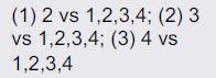
132What does the Orthogonal Helmert contrast compare?Each category except the last is compared to mean of subsequent categories
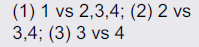
133What does the Non-orthogonal Simple contrast compare?Each category is compared to the first (or last) category
- Better to use Dunnett’s as it is corrected for comparisons made. *Simple isn’t corrected – not trustworthy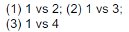
134What does the Non-orthogonal Repeated contrast compare?Each category is compared to the previous category
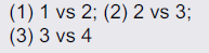
135What does the Orthogonal Difference contrast compare?Each category except the first is compared to mean of previous categories
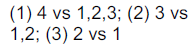
136Polynomial contrastsWhen analysing data if groups have a certain order
• Only make sense for ANOVAs where there is a logical order to the groups e.g. weight groups but NOT blood group
• Tests for TRENDS in the data, which cannot be obtained directly using post hoc tests
* Polynomial power is one lower than the group number
137Quartic trend• using polynomial to the power of 2
• gives a single curve in the line
• if there are 3 groups = quartic and linear trend
138Cubic trendline that has 2 curves in it
• if there are 4 groups = cubic trend, quartic and linear trend
139Independent factorial ANOVATwo-way design
- Two experimental factors (with levels) manipulated at same time
E.g. drug dose and mouse strain
• Compares >2 means when there are two independent variables
• NO pairing
• Can explain more of the total variability within data SO less variability left unexplained
• MORE powerful statistically than using one-way ANOVA
140Fully crossed/factorial designStudy the effect of each factor on the response variable, as well as the effects of interactions between factors on the response variable
141Balanced designEqual numbers in each group
Most power and most robustness
142Assumptions for two-way ANOVAAssumptions for two-way ANOVA are same as one-way ANOVA
1. Dependent variable that is continuous (i.e., interval or ratio level)
2. Independent variable that is categorical (i.e., two or more groups)
3. Random sampling
4. (Approx.) Normal distribution of data in each group (residuals i.e., for each level of the factor)
5. Independence of data points
6. Equality of variance among groups
143What does it mean if there is a significant interaction?• The effects of factors A & B are not independent
• Effect of one factor depends on what has happened to other factor
• Changes in dependent variable cannot be explained by independent effects of the two factors
• Makes it difficult/impossible to interpret main effects
• Do not emphasise main effects if there is a significant interaction!
144Simple effects analysisDetermine where interaction is after an interaction is found to be significant
• Analyses differences between levels of one variable (e.g., sex) at every level of the other variable(s), e.g., drug.
145How do you control for type I error rate when running a simple effects analysis?Apply a multiple comparison correction
o Choose Sidak rather than Bonferroni (too conservative – might miss an effect)
146What could be the issue with simple effects analysis?Doesn't provide a truly accurate result, as it doesn't take into account the interaction between variables
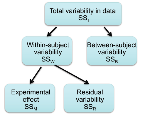
- provides good cause of interation
147Within-subject variabilityDifferences between conditions within subject
148Between subject variabilityVariability between mean levels across conditions for each of those subjects
149How is repeated measures ANOVA broken down?Looks at within subject variability only and ignores differences between individuals to identify common changes
150Repeated measures ANOVA assumptionsSame as one-way ANOVA:
o Normality of residuals
o Sphericity = Instead of equality of variances from mean of each group, we need equality of the differences between linked values in each group.
151Repeated measures ANOVAWhen data is not independent - Linked values
• Paired t-test to 3 or more groups
- Can follow up repeated measures with a multiple comparisons test
• If parametric assumptions fail, use the nonparametric equivalent, Friedman test.
152Mauchly's TestTest for sphericity
Used to validate a repeated measures ANOVA
153What issues with data limit the ability to interpret results?DON'T PUT SPHERICITY
- not a limitation can always be fixed
? ANSWER ?
154What does it mean if Mauchly's test is significant?Sphericity can’t be assumed and the significance from the F ratio is inaccurate.
• Violation of sphericity has bad effects on accuracy of multiple comparison tests.
• Bonferroni test is the most robust.
155What is sphericity?Equality of the differences between linked values in each group.
Variance between all possible pairs of within-subject conditions are equal
- like Levene's test
• F ratio inflated
• increase in the Type I error rate
156Greenhouse-Geisser correctionIn Mauchly's test for sphericity:
• adjusts degrees of freedom, which changes significance level associated with F statistic – doesn’t adjust F ratio
• Too conservative – p value higher than it should be
157Example of repeated measures ANOVAWeight gain over 2-week period for 8 rats fed each of four diets (counterbalanced order)
158Counterbalanced orderRemoves potential confounds
• E.g. removes the effect of time over the effect of diet if each animal is fed each of four diets over 2 weeks
159How to interpret Mauchly's test of sphericity?• If significance >0.05 assume sphericity
- Quote from sphericity assumed line
• If significance <0.05 can't assume sphericity – must apply a correction:
- Greenhouse-Geisser and Huynh-Feldt
160Huynh-Feldt correctionIn Mauchly's test for sphericity:
• bit too liberal – p value lower than it should be
161Rules for interpreting the Greenhouse-Geisser and Huynh-Feldt corrections?Look at GG and HF values in epsilon
- If GG is above 0.75 then you take HF
- If GG is below 0.75 then you take GG
Quote data from the correction's line
162How to work out the DF for the GG and HF?Epsilon value GG * total DF = GG DF
- Reduces DF associated with model and error DF to reduce significance associated with F ratio
163Repeated measures factorial ANOVAWhere there is more than one factor and they are repeated measures, e.g., Two-way repeated measures ANOVA.
• Test for interactions between factors like independent factorial ANOVA.
164Sidak correctionCounteract multiple comparisons problem and control familywise error rate
Correction for SIMPLE EFFECTS analysis
• Independent comparisons
- non-repeated factors
165Assumptions of Repeated measures factorial ANOVA• Sphericity like repeated measures ANOVA
• Parametric - no non-parametric equivalent
166Friedman testNon-parametric equivalent of a single factor repeated measures ANOVA
167Mixed model ANOVAFactorial design with at least one independent factor and at least one repeated measures factor
• e.g. Sex x strain x drug (where drug is repeated measures)
168Mixed model ANOVA AssumptioinsMix of repeated measures and independent factors = mix of assumptions:
o Equality of variance assumption of independent ANOVA
o Sphericity assumption of repeated measures ANOVA
169Planned contrasts and simple effects post-hoc analysis for mixed model ANOVACan break down ANOVA into individual comparisons of interest
- Use BONFERRONI for comparisons of repeated measures
- SIDAK correction for independent comparisons
170Bonferroni correctionControl for multiple comparisons problem and familywise error rate
• Comparisons of repeated measures
Corrects P value by dividing by number of tests
171Polynomial regression• Adding further terms to polynomial will automatically improve fit, (increase R2)
172Over-fitted curveFit to data is very good but not a good model because it fits random variability which would not generalise and influenced by random fluctuations
173Non-Linear regressionWhen the relationship cannot adequately modelled with linear parameters
• Fit a curve to the data based on established theoretical relationship
• Cann't calculate R2 for non-linear regression
• Must have curves in residual/ scatter plots
174HillslopeDescribes the steepness of the family of curves
o At point of invariance ??
o Constrain HS to a constant value of 1.0
175Type I errorFalse Positive
• When the null hypothesis is true and you reject it
• Probability of making a type I error is α (p value)
• To lower risk, lower α value
--but less likely to detect a true difference
176Type II errorFalse Negative
• When null hypothesis is false but fail to reject it
• Probability of making a type II error is β (test power)
• To lower risk, increase power by increasing sample size
e.g. Type II error rate 20% = 20% chance of missing an effect
177Individual error rate?• Max probability that one or more comparisons will incorrectly conclude significance
178Resampling stastiticsNon-parametric tests that make no assumptions about data distribution other than sample is representative of population
• Used in place of an unpaired t-test or One-way ANOVA if parametric assumptions aren’t met
• More powerful than non-parametric as size of differences retained
179Permutation testTests for differences between means (or medians)
o Sampling WITHOUT replacement to test hypotheses of “no effect”
180How does a permutation test work?i
181BootstrappingMore ROBUST resampling procedure that allows CI and SEM for means/medias to be derived without assumptions for population distribution
• Sampling WITH replacement
182Assumptions of Non-linear regressionSame as simple linear regression:
• Independence of data points
• No significant variability in predictor
• Normal distribution of residuals
• Homoscedasticity (equality of variance)
• Value of X not used to compute Y – no entanglement of variables
183How do we compare models?- Can’t simply compare R2 values, have to analyse differences in residuals of the two models
- The higher the SS the less unexplained variability by the model
184How does the DF change if you constrain a parameter?Add another DF
185What do you do if the criteria for use of chi squared are not satisfied i.e., >20% of E<5?• Combine 2 (or more) rows or columns of contingency table in a way that makes scientific sense
• Otherwise, Fishers exact test
186How does Bootstrapping work?Sampling WITH replacement
1. Take sample from group, calculate statistic
2. Replace sample and repeat thousands of times
187Adjusted R2How well model generalises explained variability i.e. how well it fits a different sample from same population