Description
|
|
Created by Rohit Gurjar
over 7 years ago
|
|
Page 1
Introduction
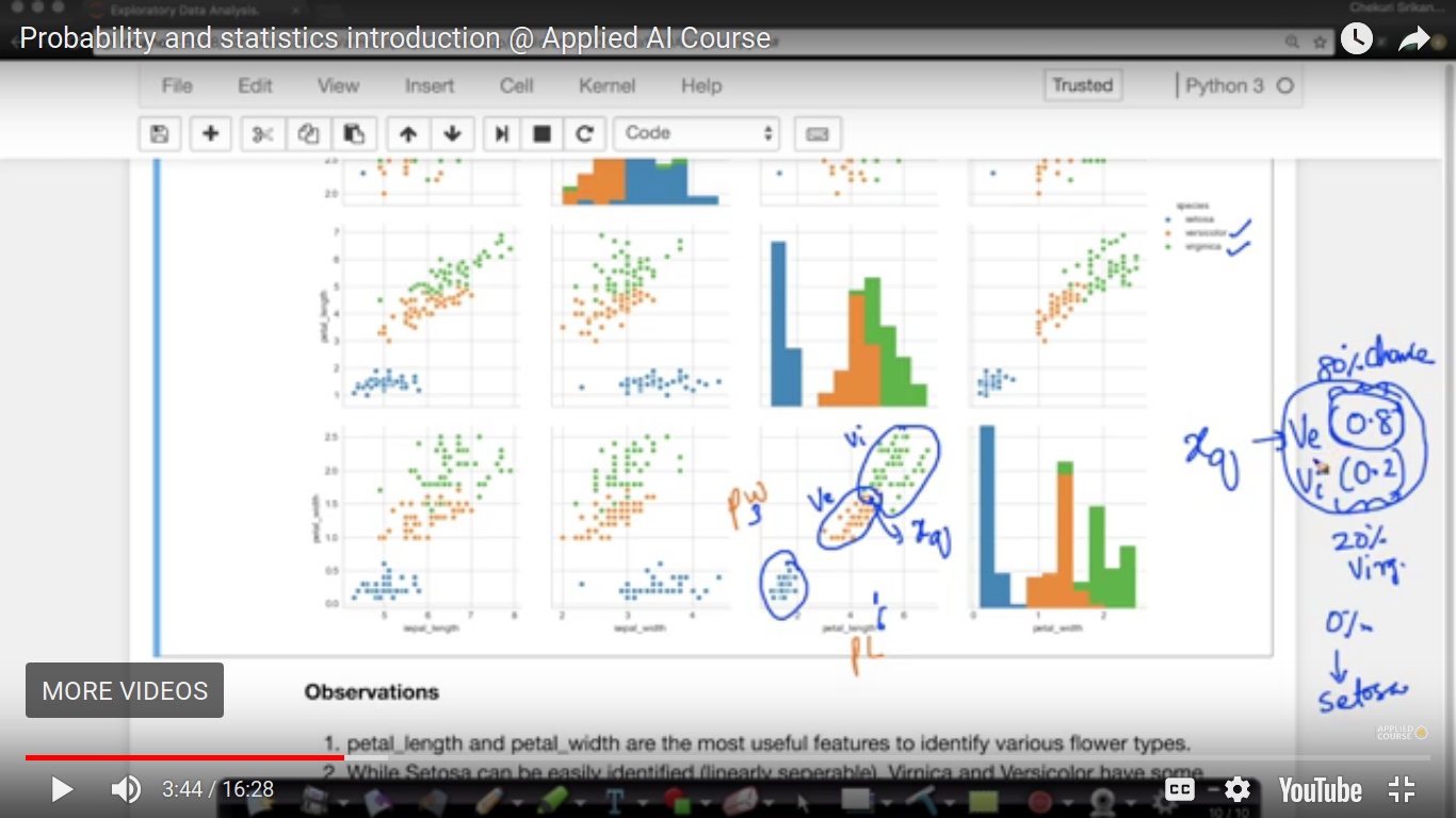
This is a scatter plot between petal width as the y-axis and petal length as the x-axis from the IRIS dataset. The setosa flower is well separated but let us suppose picked some random point(xq, where q is the query point) which here is the intersection of versicolor and verginica. So, the prediction of the type of xq is not easy. So, here we are using probabilistic score to predict it.
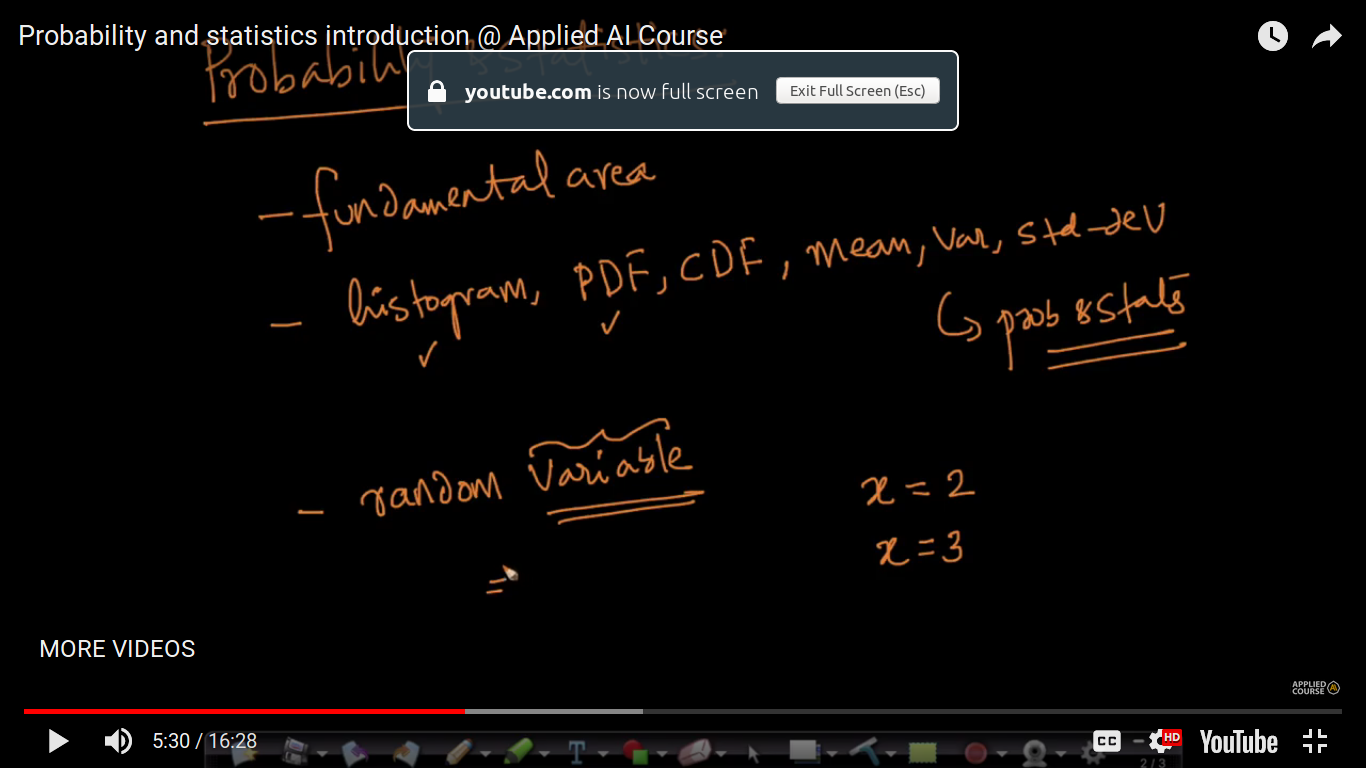
Here are all the concepts shown used in probability section and discussed in detail. P(X=x1) or P(x1)
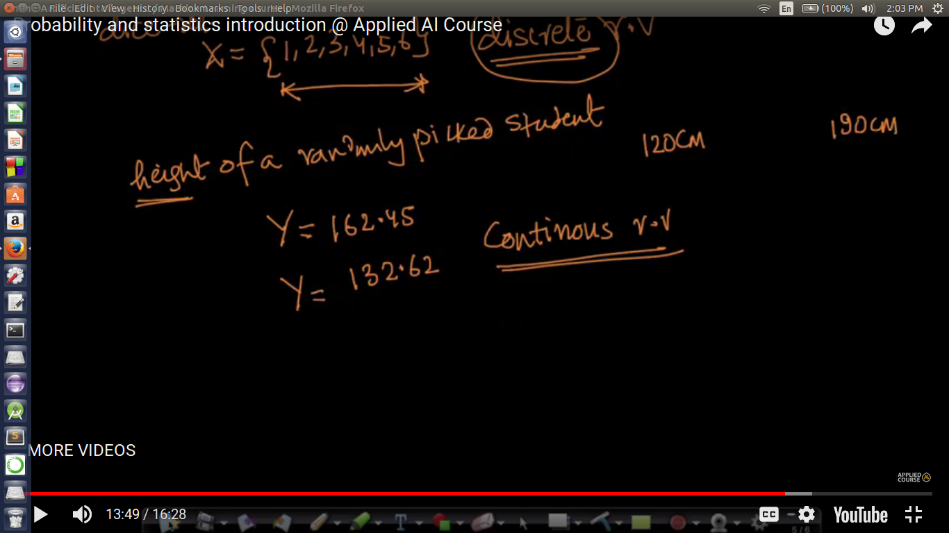
Discrete Random Variable - When a random variable can take one value from a finite set of items or values. Continuous Random Variable - A random variable which can take any real value.
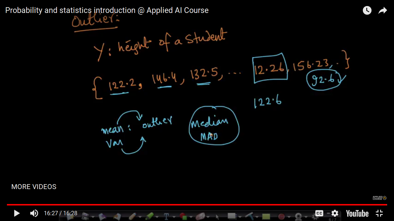
Outliers in Probability : A highly differentiated value from a set of values or observations. Here is the prediction of heights which mostly lies in the range of 120-190cm but value 12.26(from human error 122.6), 92.6 (which may be found that height but act as an outlier in this dataset).
Page 2
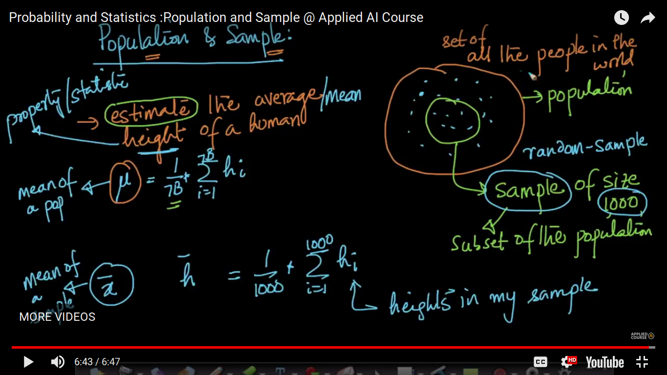
Population & Sample
Population - Set of all the events or observations Sample - Sample is the subset of the population which we have taken to make an estimate. Here height is the property or statistics.
Page 3
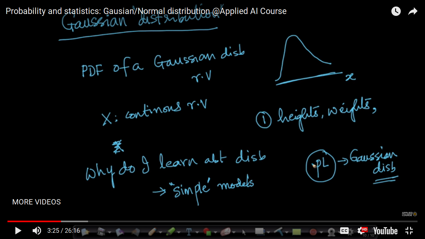
Gaussian & Normal Distribution and it's PDF
PDF: Probability Density Function
Why do I learn about Distribution? Distributions are a very simple model of natural behavior. For Example: If the petal length follows the Gaussian distribution, we can tell the bunch of properties such as length, width, height etc about petal length without having to measure any of the petal lengths.
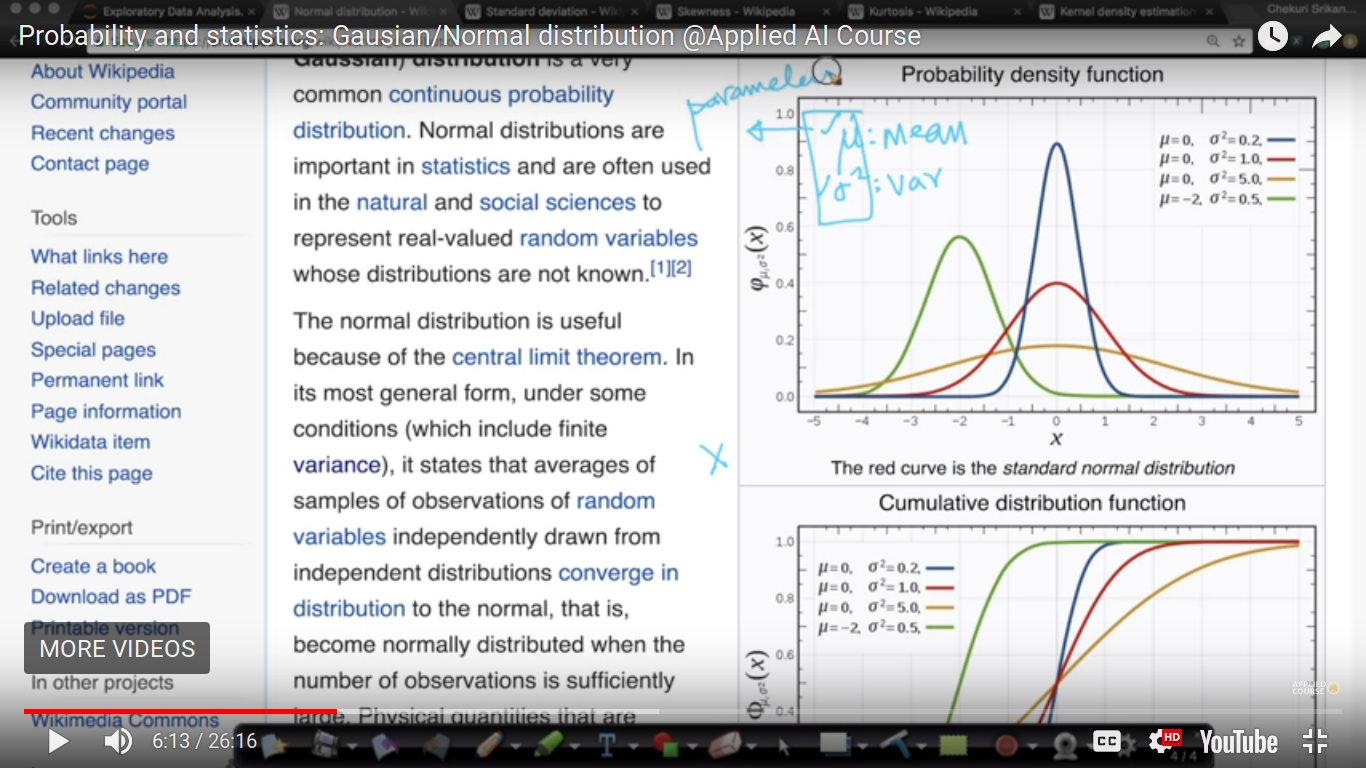
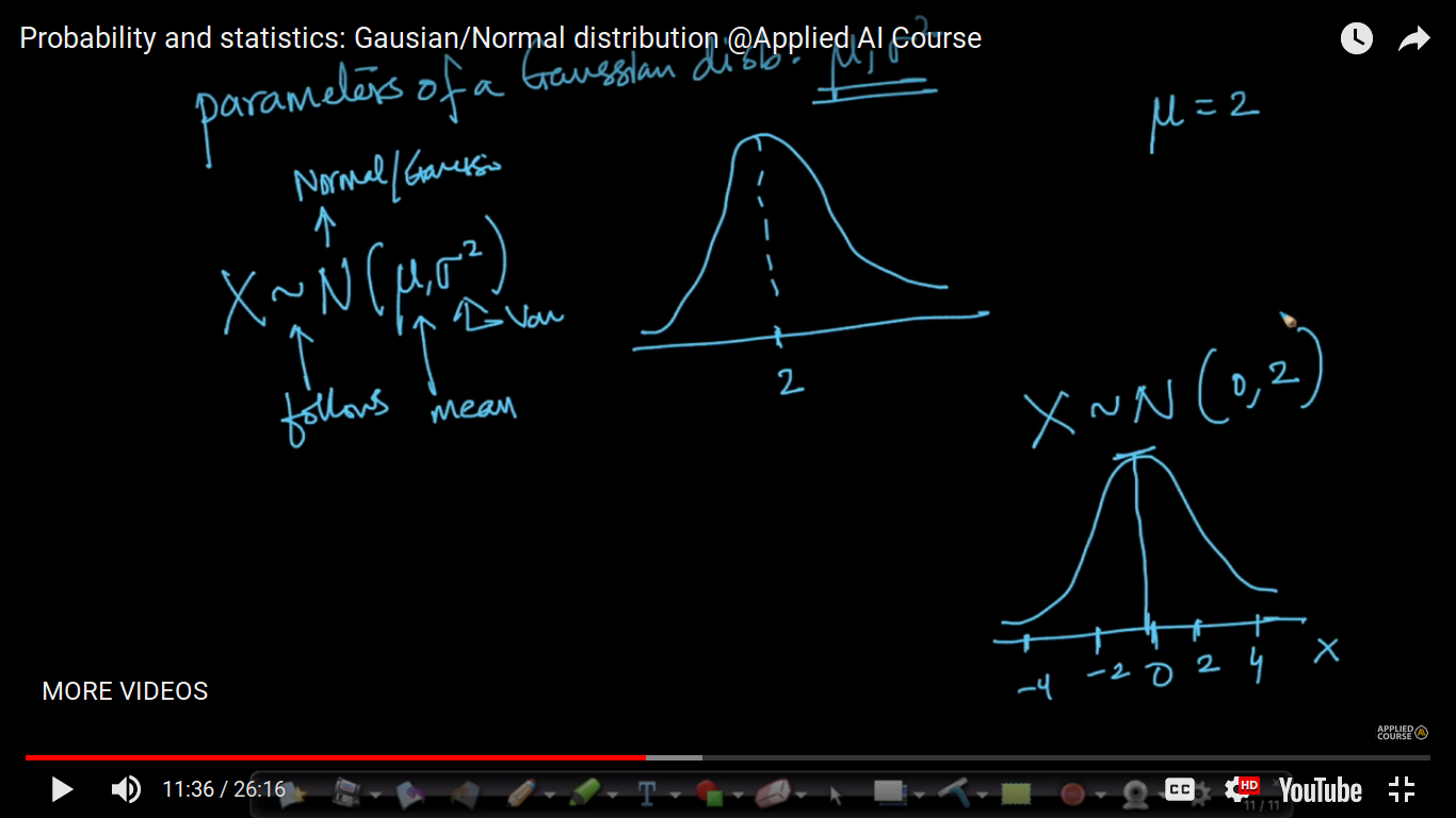
parameters of the Gaussian distribution: mu(mean) and sigma^2(variance) If we have mean and variance, then we can le to tell about everything about the probability density function of the Gaussian distributed random variable.
Here, mu(mean) and sigma^2(variance) are the parameters of the distribution. If X follows a Gaussian distribution and parameters are given, then we can easily determine its PDF of distributed random variable and then it's CDF.
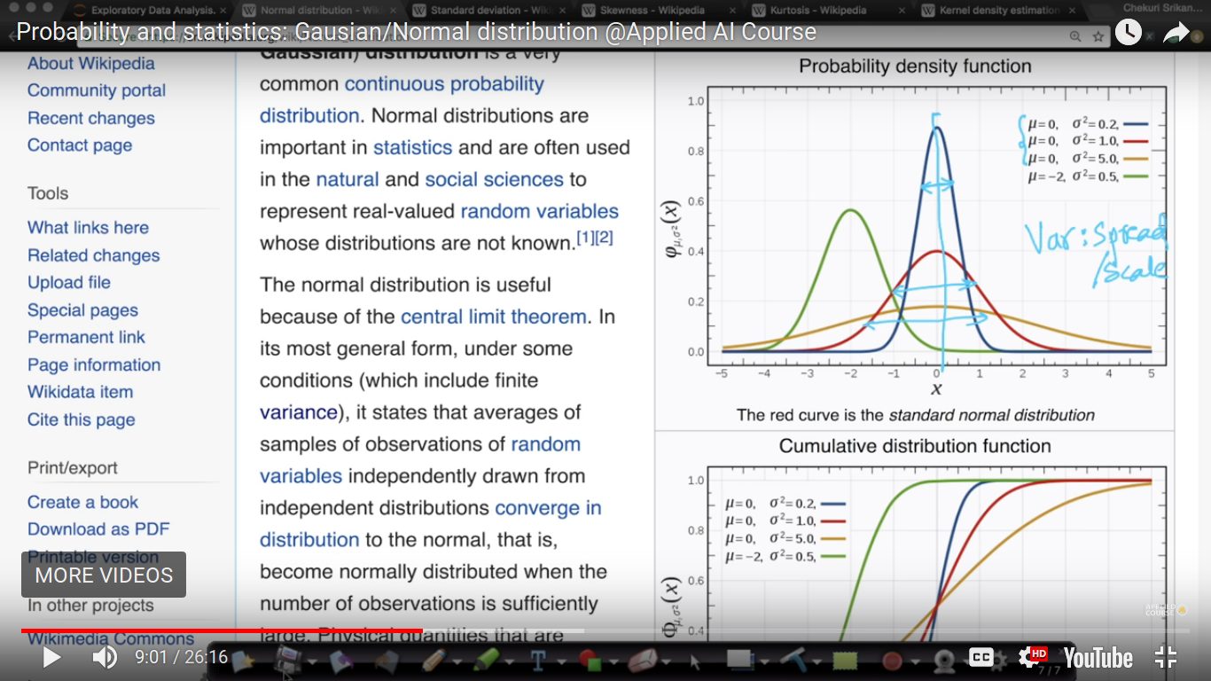
Here, width represents the variance. Variance is a measure of spread. The peak of the Gaussian distribution is at mu(mean).
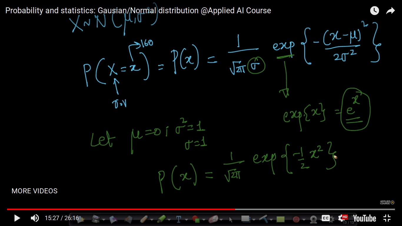
If X follows Normal Distribution then the probability of a random variable, x is given by above formula -
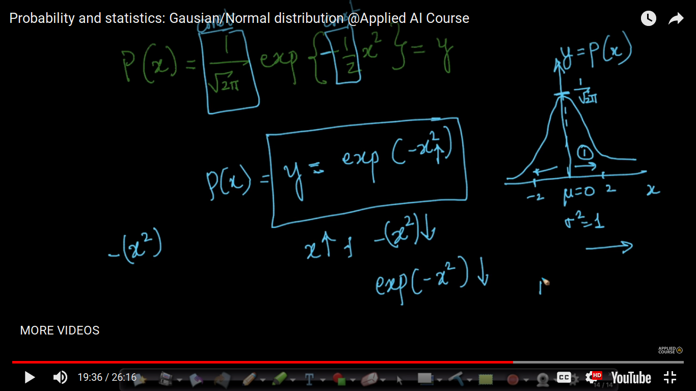
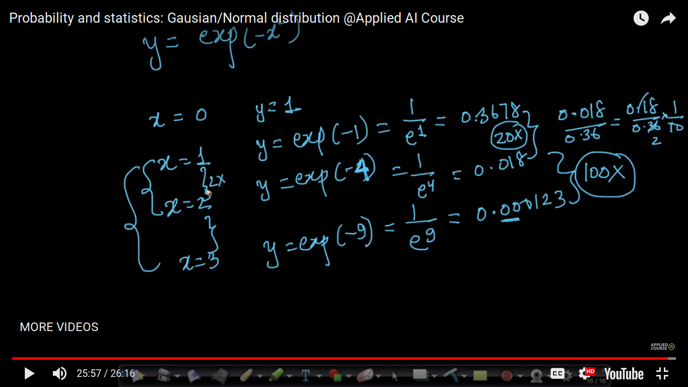
If x is increasing then the probability of normal distribution is drastically decreasing. It's about decreasing to the exponential to the power 2.
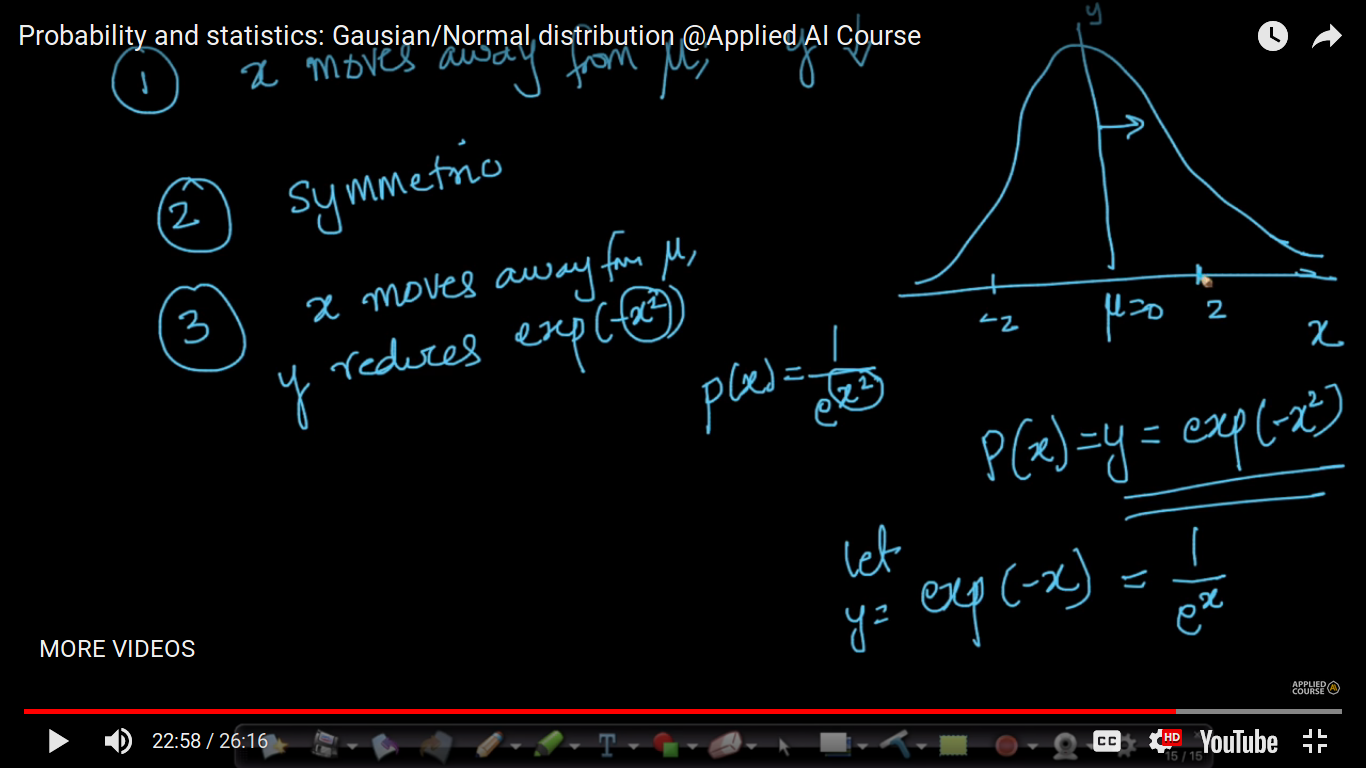
The conclusion of the above graph-
Page 4
Cumalative Distribution function
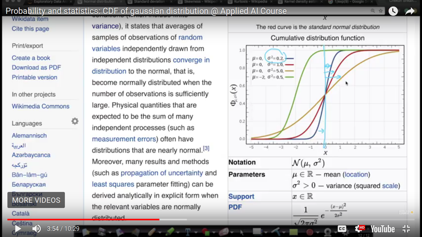
CDF graph is having half side on the left side of the mean and the half on the right side. Here, if the variance is less then it means it is closer to the x=0 line.
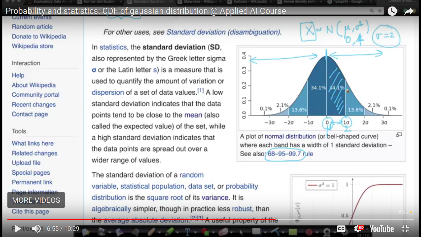
Here, is the 68-95-97 rule for the distribution of the population.
Page 5
Symmetric Distribtn, Skewness,Kurtosis
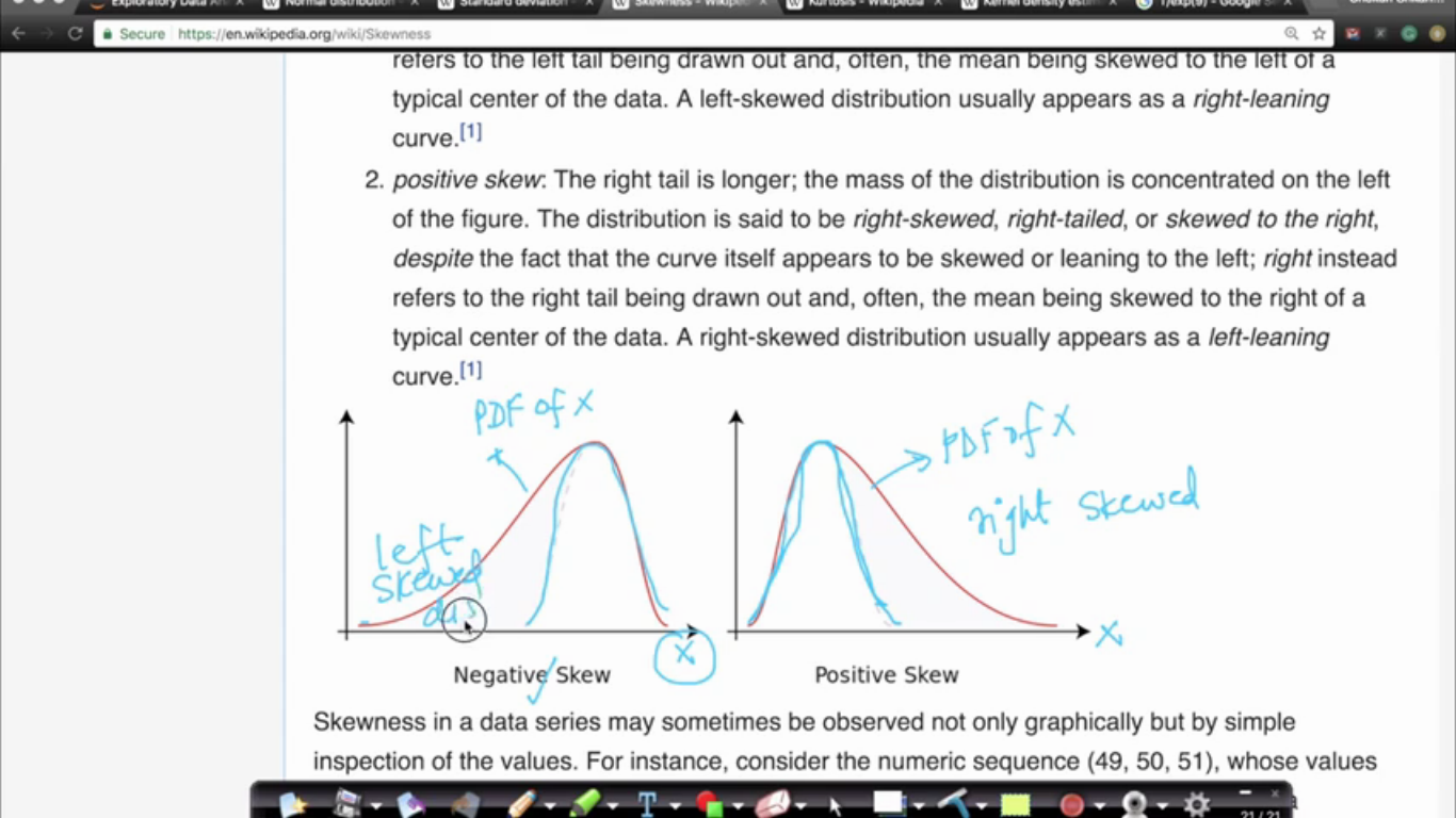
Skewness: How dissimilar is the distribution as compared to the symmetric distribution.
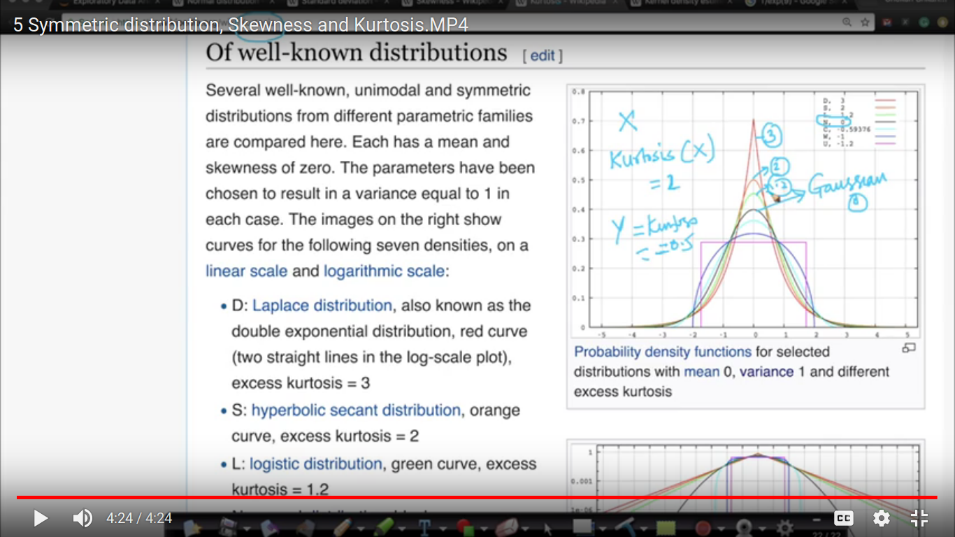
Kurtosis: Kurtosis measured peakeredness of the distribution.
Page 6
Standard Normal Variate
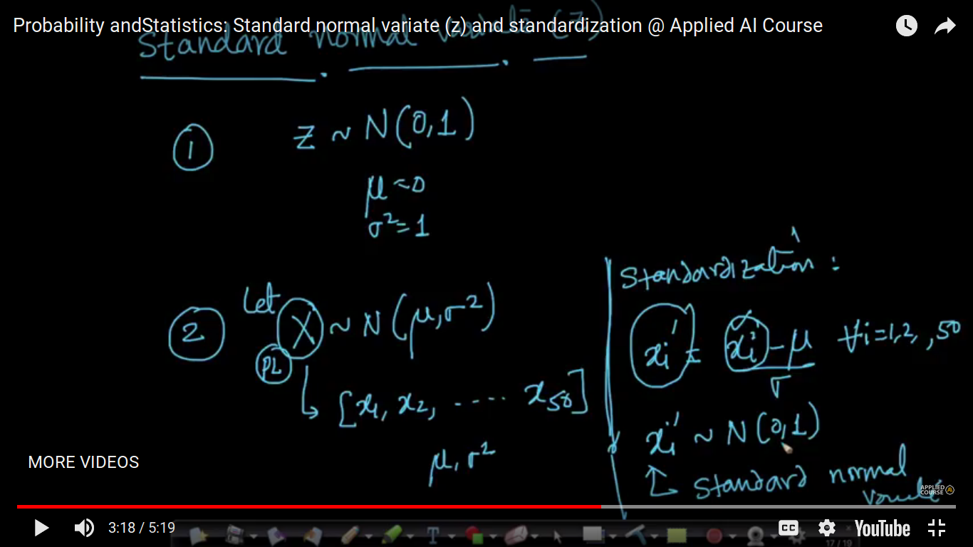
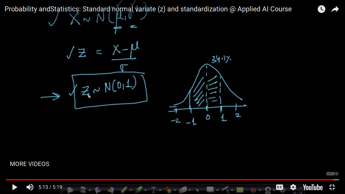
'Z' here represents a random variable. Why are we using Standard Normal Variate? Because after standardized the data, my 34.1 % of the data lies between 0 and 1.
Page 7
Kernel Density Estimation
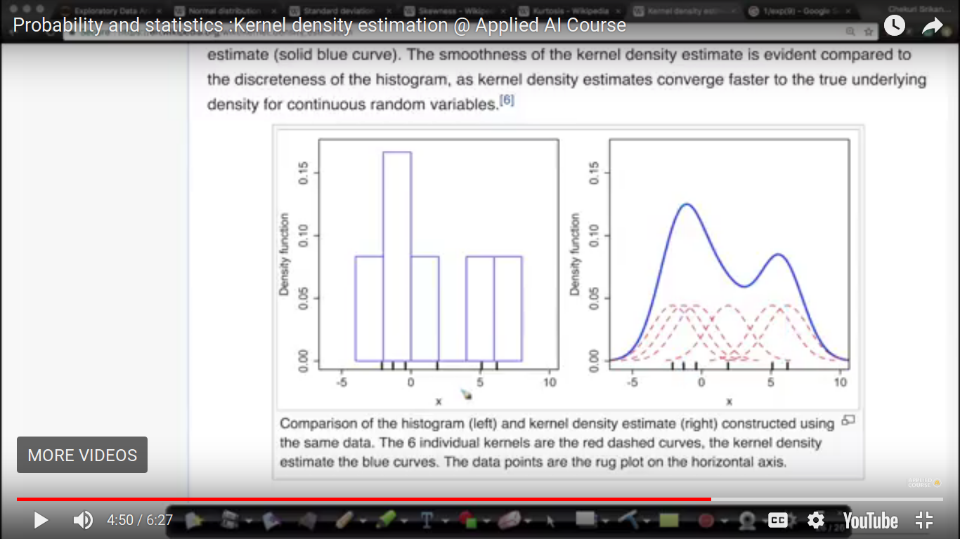
1. KDE is one way to smooth a histogram. Smoothed functions are easier to represent in functional form i.e., as f(x) as compared to non-smooth functions. Additionally, smooth functions represented as f(x) as easier to integrate. We need integration as CDF is an integration over PDF. Smooth functions represented in functional form are easier to manipulate to build more complex operators on the data. 2. KDE is used to obtain a PDF of an r.v. Histograms and PDFs inform of the density of data for each possible value an r.v takes. We have explained about PDFs and their interpretations in details in the above videos in EDA especially in this one: https://www.appliedaicourse.com/course/applied-ai-course-online/lessons/histogram-and-introduction-to-pdfprobability-density-function-1/ If we decrease the window size and increase the number of bins then the graph of PDF becomes zagged like structure This is the kernel density gaussian kernels. ## Yes, the variance for these Gaussian kernels is a parameter which we can tune based on our need for smoother or jagged PDFs. If we keep the variance very small, we get a very jagged PDf and if we keep it too wide, we get a useless and flat PDF. So, it is a tradeoff. In practice, most of the plotting libraries use rules-of-thumb or various algorithms to determine a reasonable variance. For example in SciPy, the bandwidth parameter determines the variance of each kernel. There are many methods to determine the bandwidth parameter as per this function reference: https://docs.scipy.org/doc/scipy/reference/generated/scipy.stats.gaussian_kde.html
Page 8
Sampling Distribution & Central Limit Theorem
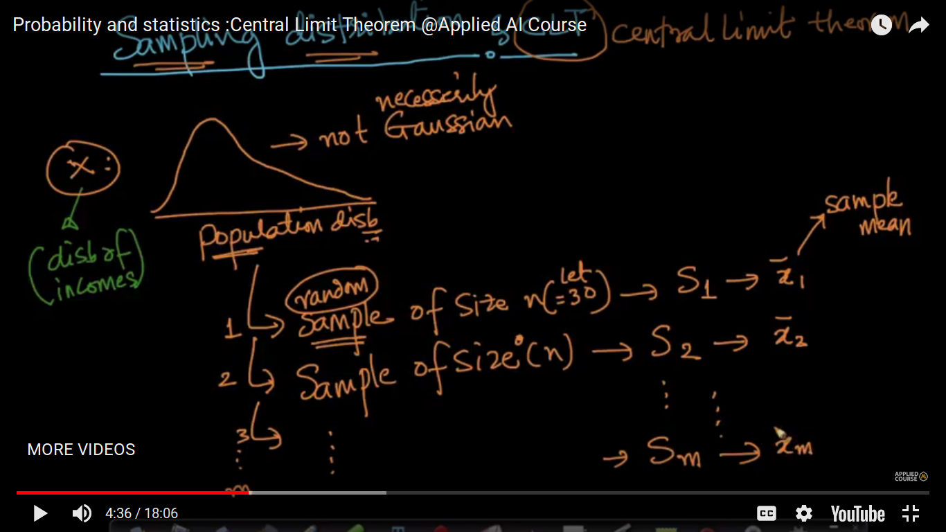
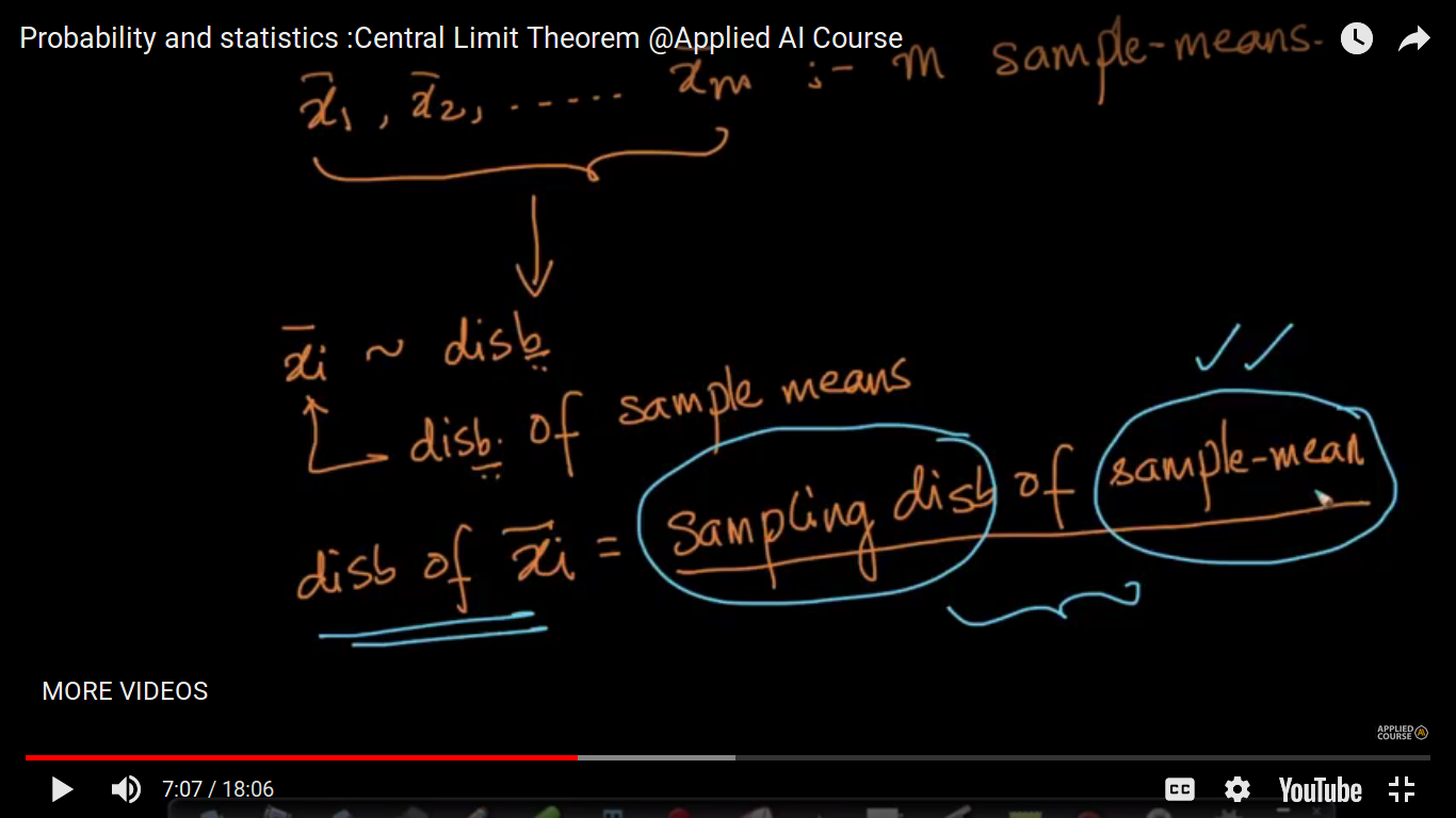
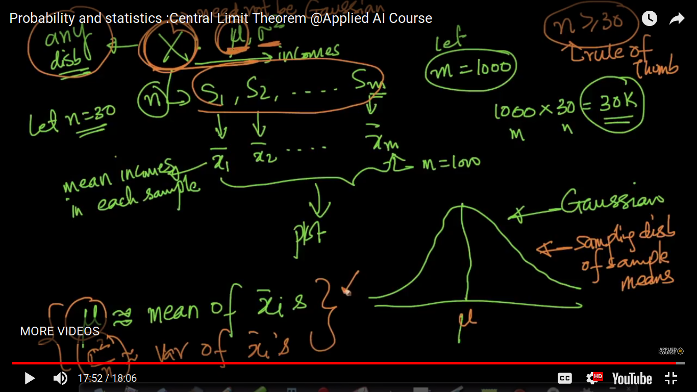
The central limit theorem states that if you have a population with mean μ and standard deviation σ and take sufficiently large random samples from the population with replacement, then the distribution of the sample means will be approximately normally distributed. This will hold true regardless of whether the source population is normal or skewed, provided the sample size is sufficiently large (usually n >= 30). If the population is normal, then the theorem holds true even for samples smaller than 30 Distribution implies PDF(Probability Distribution Function) In practice, you do not get to see the all the values of a population. Let us say, you want to estimate the mean height of all humans. It is impossible to have the height of each of the billions of humans in your dataset. What we obtain is a sample of hights of a subset of humans. Now, that is why sample-means are useful and important. Even for a dataset, you do not see the features values for every datapoint int he universe. What you see as a training dataset is only a sample of points.
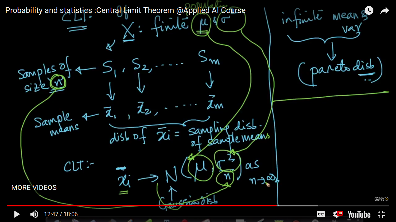
Please note that we can never get out hands on the population data in most real-world cases as the data may be too large or too hard to obtain. So, CLT helps us estimate the population mean reasonably well, using samples from the population, which are easier to obtain. No, we are not trying to cross-check the mean. We are trying to estimate the population mean given the sample means. Please note that a “sample” is a subset of observations from the universal_set/population of data-points. The most important result about sample means is the Central Limit Theorem. Simply stated, this theorem says that for a large enough sample size n, the distribution of the sample mean will approach a normal distribution. This is true for a sample of independent random variables from any population distribution, as long as the population has a finite standard deviation (sigma). Central Limit Theorem is that the average of your sample means will be the population mean. In other words, add up the means from all of your samples, find the average and that average will be your actual population mean. Similarly, if you find the average of all of the standard deviations in your sample, you’ll find the actual standard deviation for your population it’s applicable to any general distribution of the random variable. distribution of the sample means will be approximately normally distributed. This will hold true regardless of whether the source population is normal or skewed
Here, we can easily compute the mean and variance of the distribution, X using PDF. if n>=30, then any distribution behaves as a normal or Gaussian distribution. The mean and variance of xi bar become slightly equal to the population Mean and variance/n respectively where n is tending to infinity. https://stats.stackexchange.com/questions/44211/when-to-use-central-limit-theorem
Page 9
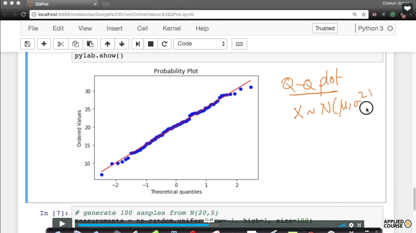
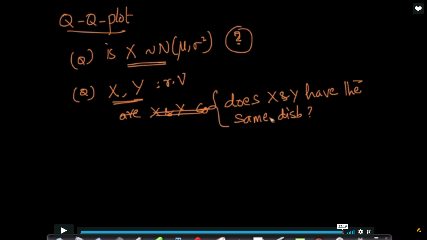
Q-Q Plot - How to test if a random variable is normally distributed or not?
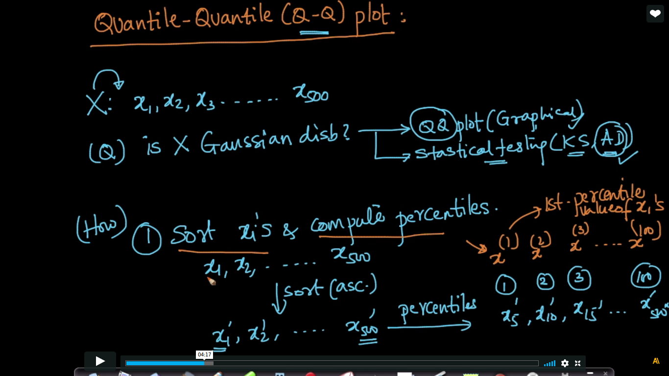
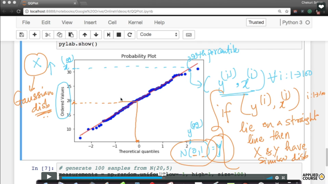
AD - Anderson Darling(Strongest test to determine Gaussian distribution) Q-Q plot is generally used to understand whether the random variable is Normal or Gaussian distributed or not X, Y- random Variable
In this video.. how to do Q-Q plot shown and compute percentiles is best shown in Exploratory Data Analysis.
So, the point corresponding to the '0' is roughly the mean because Here, points are drawn with the percentiles.
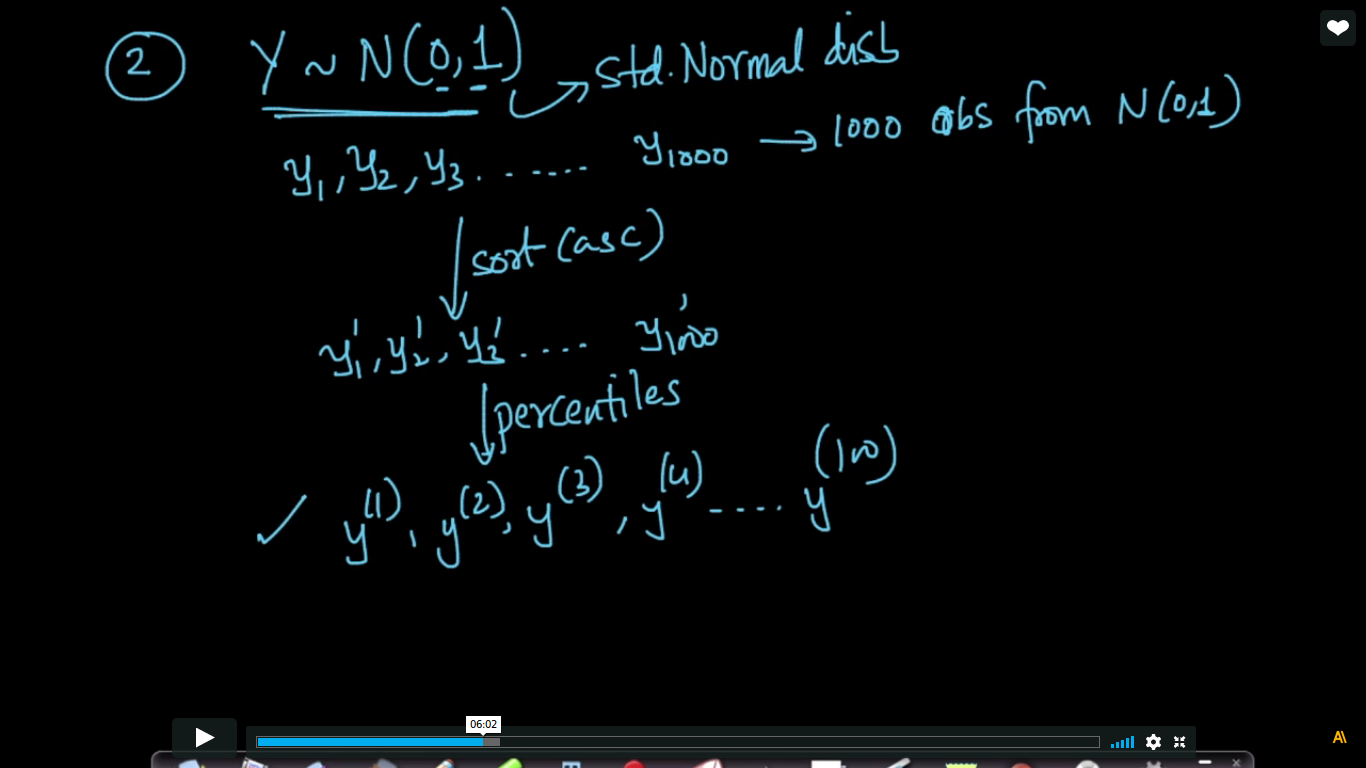
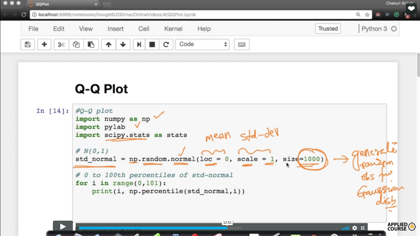
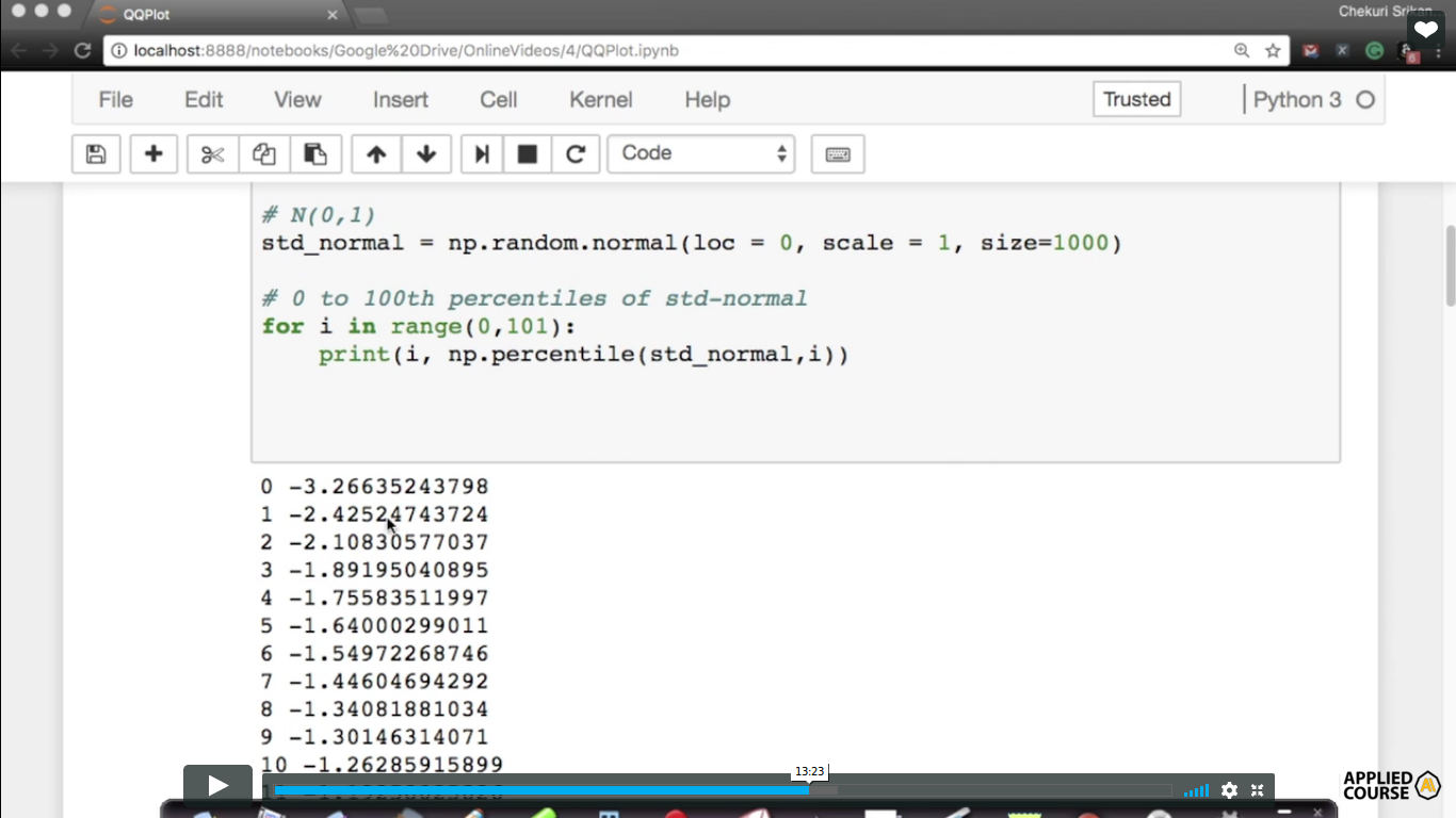
Generate random numbers from a normal distribution with mean 0 and std-deviation 1and generate 1000 such samples and all that put into a single variable( std_normal). So, this is how you generate random observations from the Gaussian distribution. then find the percentiles from 0 to 100.
We find out the percentiles of the samples.
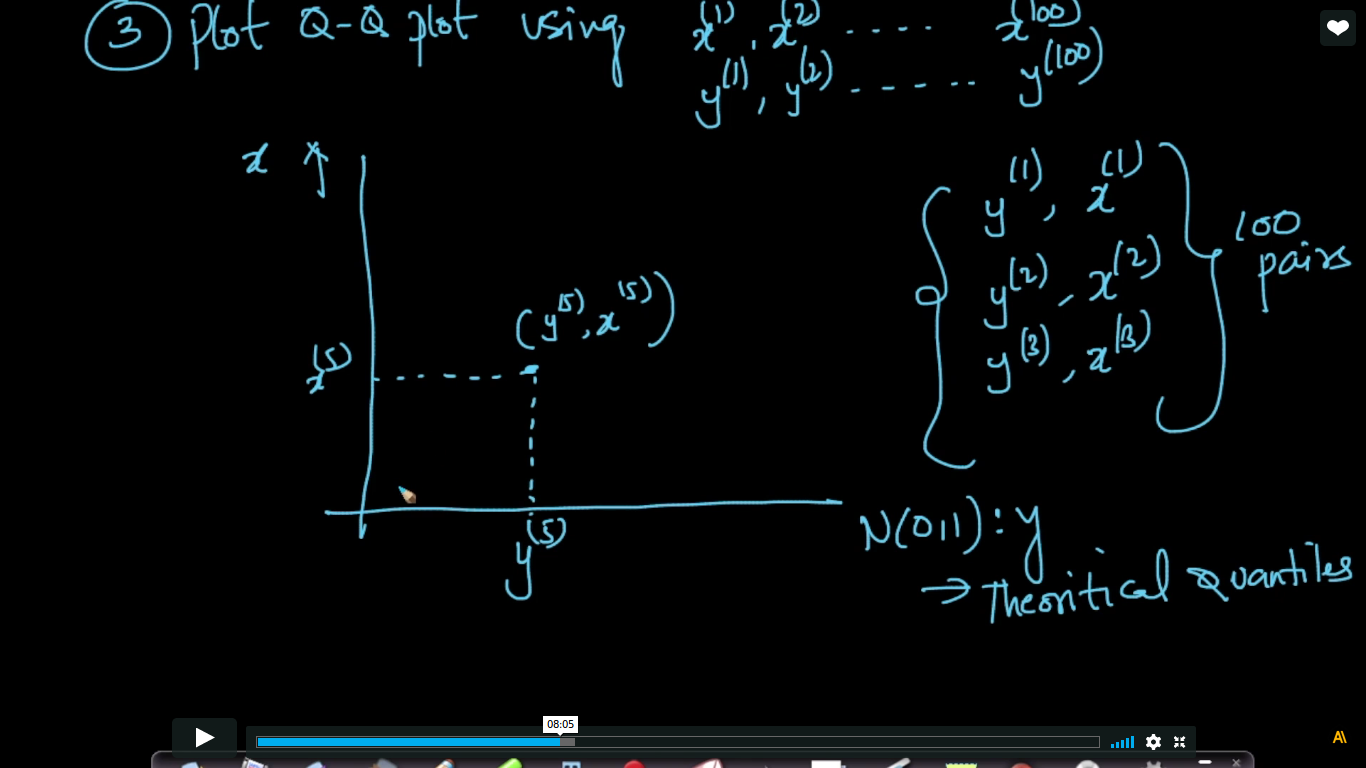
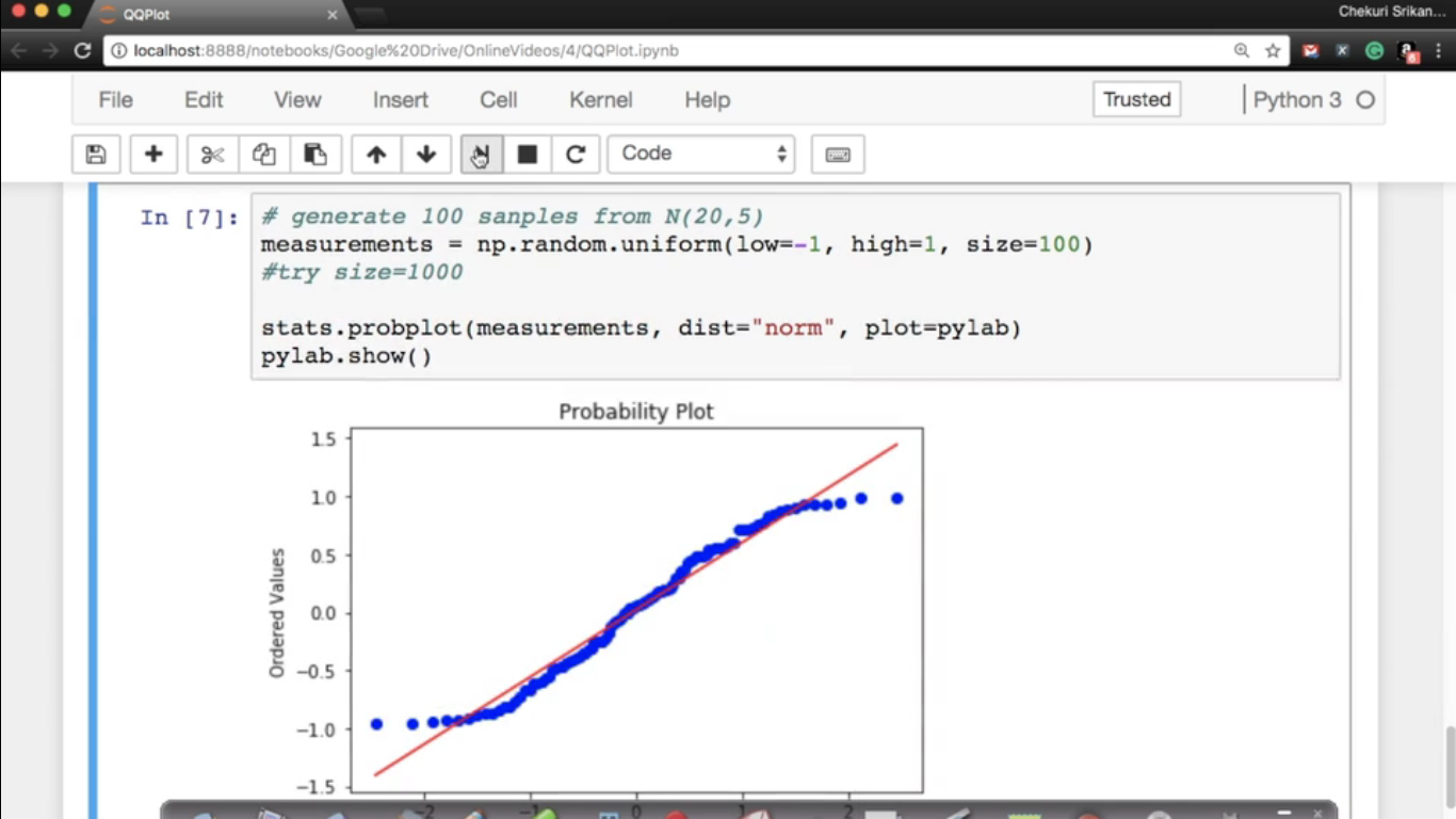
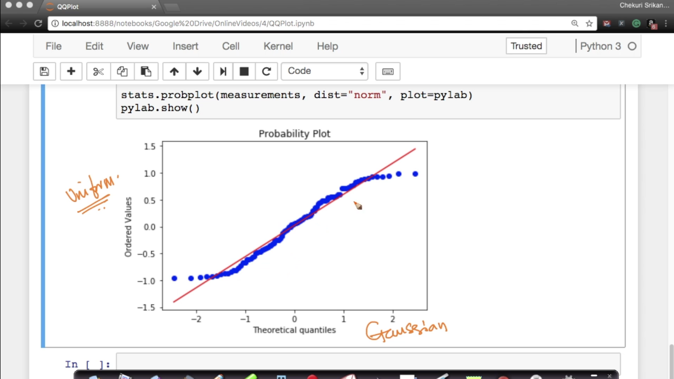
Using prob plot, we are comparing our measurements of samples with the standard normal variate.
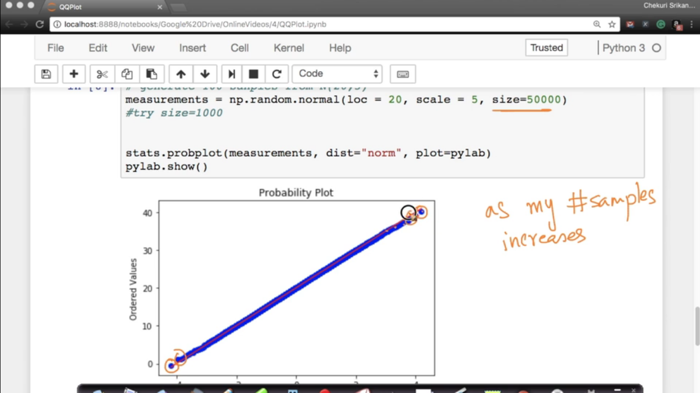
As my samples increases, the points are moving towards more closer and closer to the straight line.
Why we need Quantile-Quantile plot? Here, Y need not be a normal distribution.
measurements = np.random.uniform(low=-1,high=1,size=100) In this case, points are diverging at the extremeties because they are belong to the different family.
Page 10
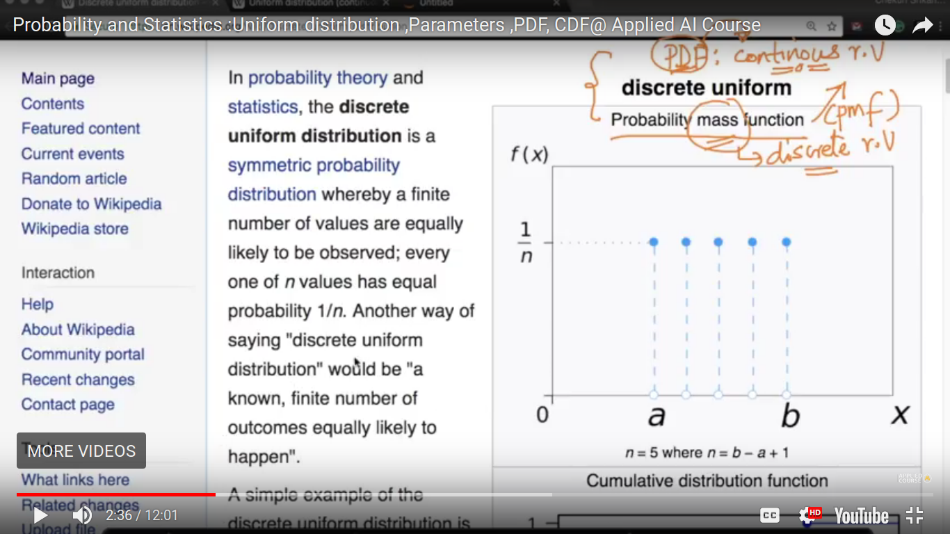
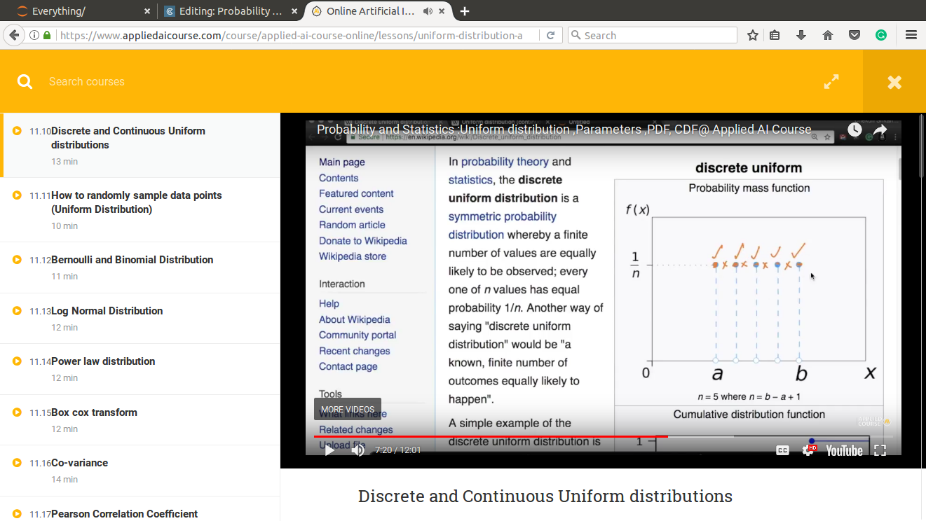
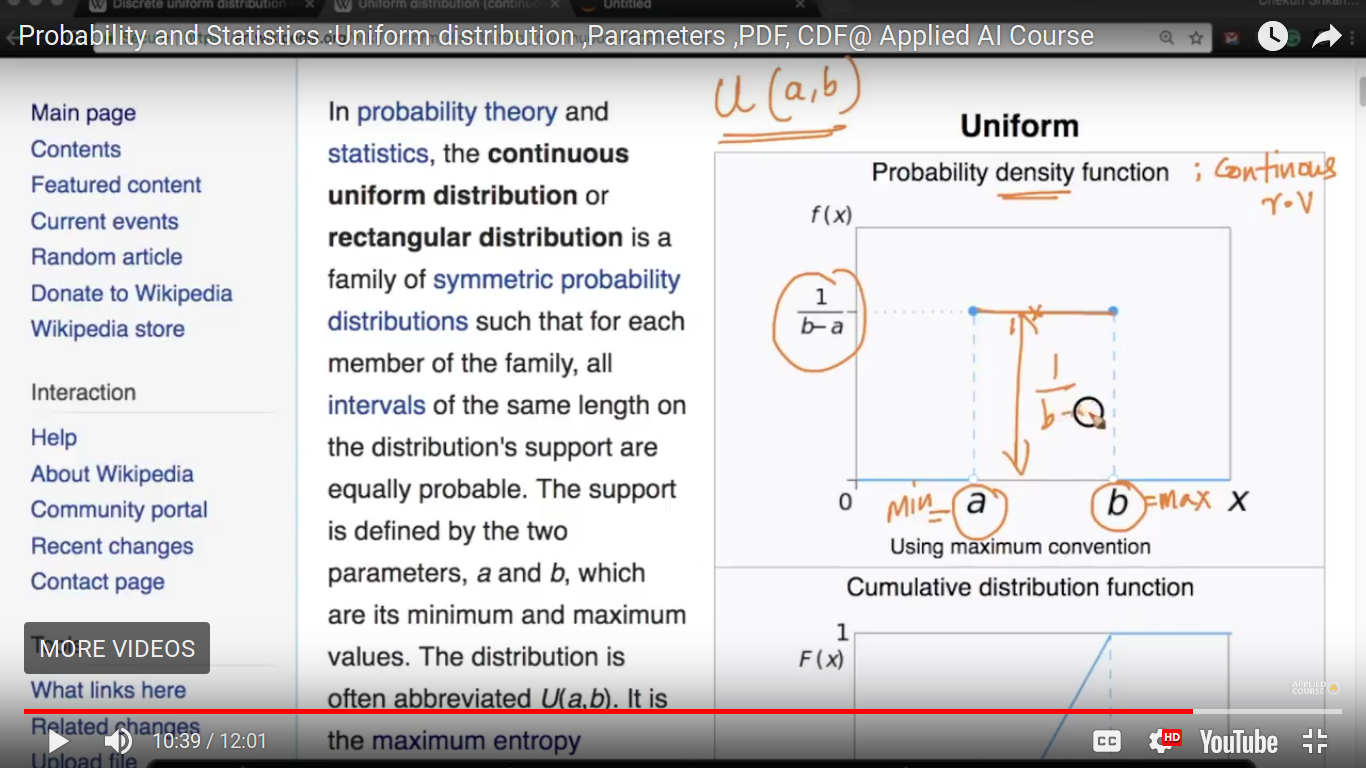
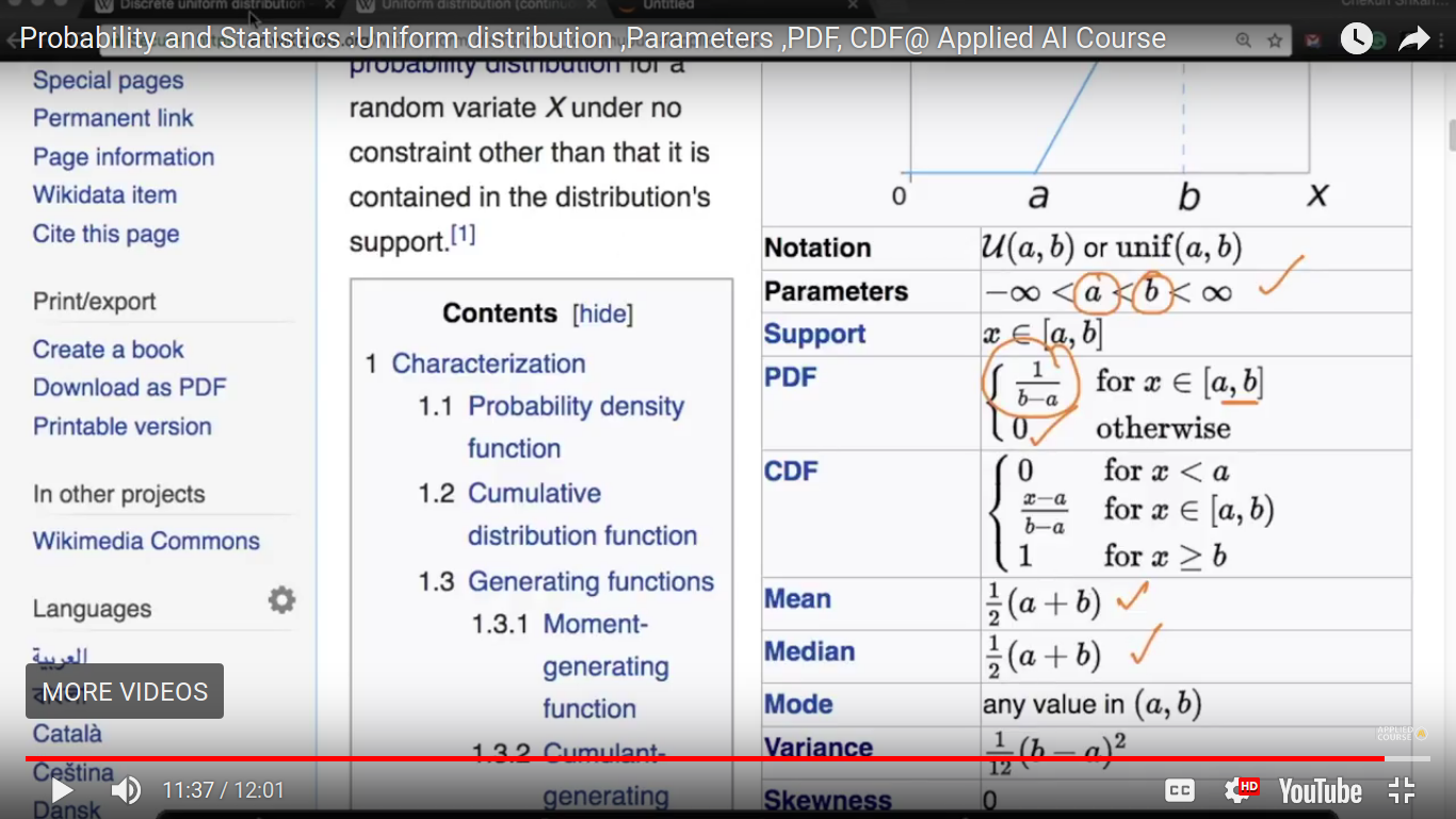
Uniform Distribution
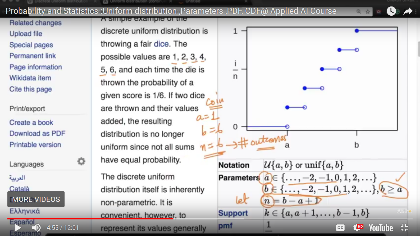
#outcomes = no. of outcomes and they are equally probable in the above example.
The probability of each of the points is equally probable and is equal to 1/n where n = b-a+1 And probability mass function is determined for a discrete random variable. So, there is no probability in between integers.
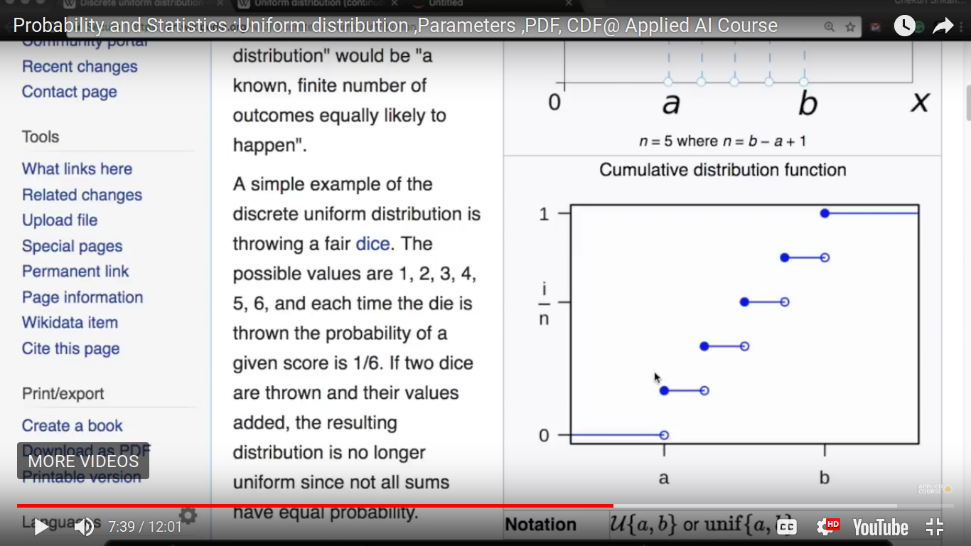
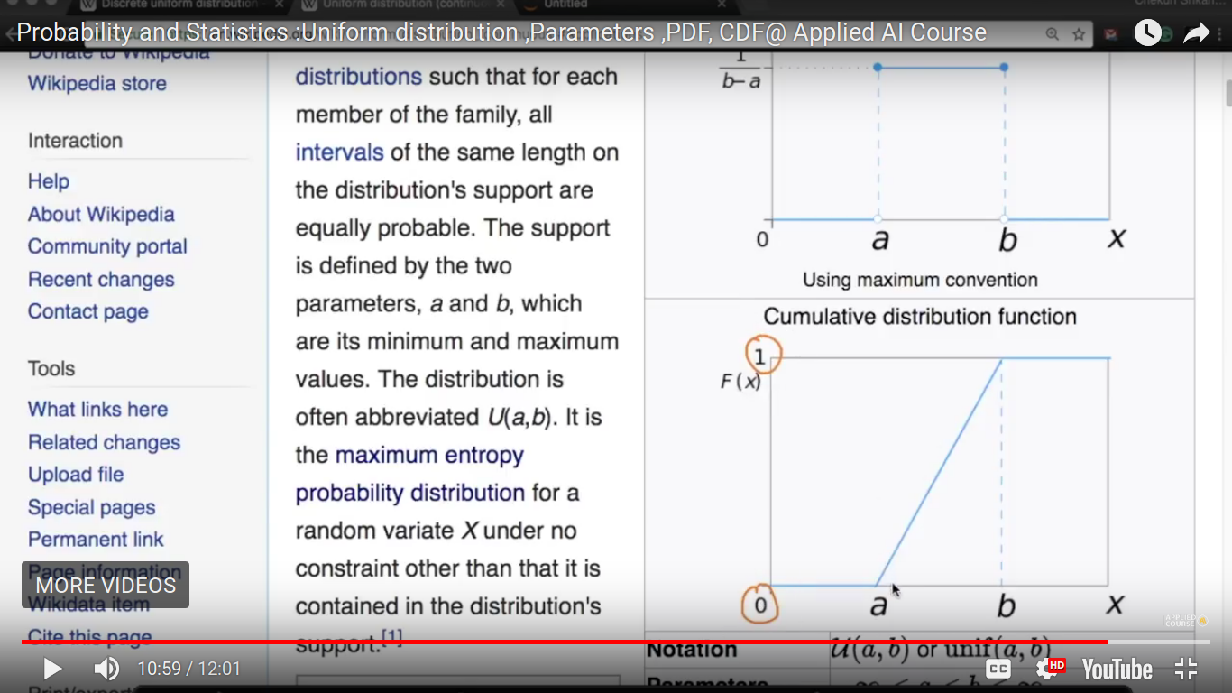
CDF of a uniform discrete function.
Page 11
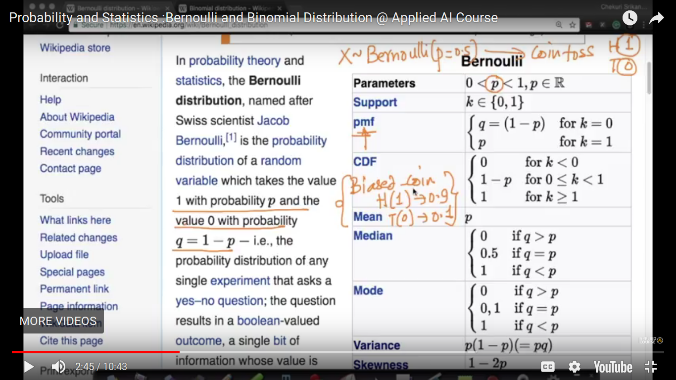
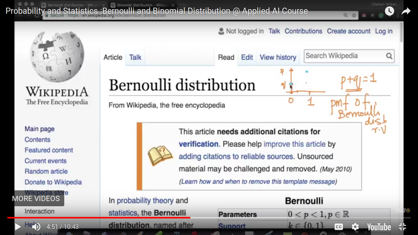
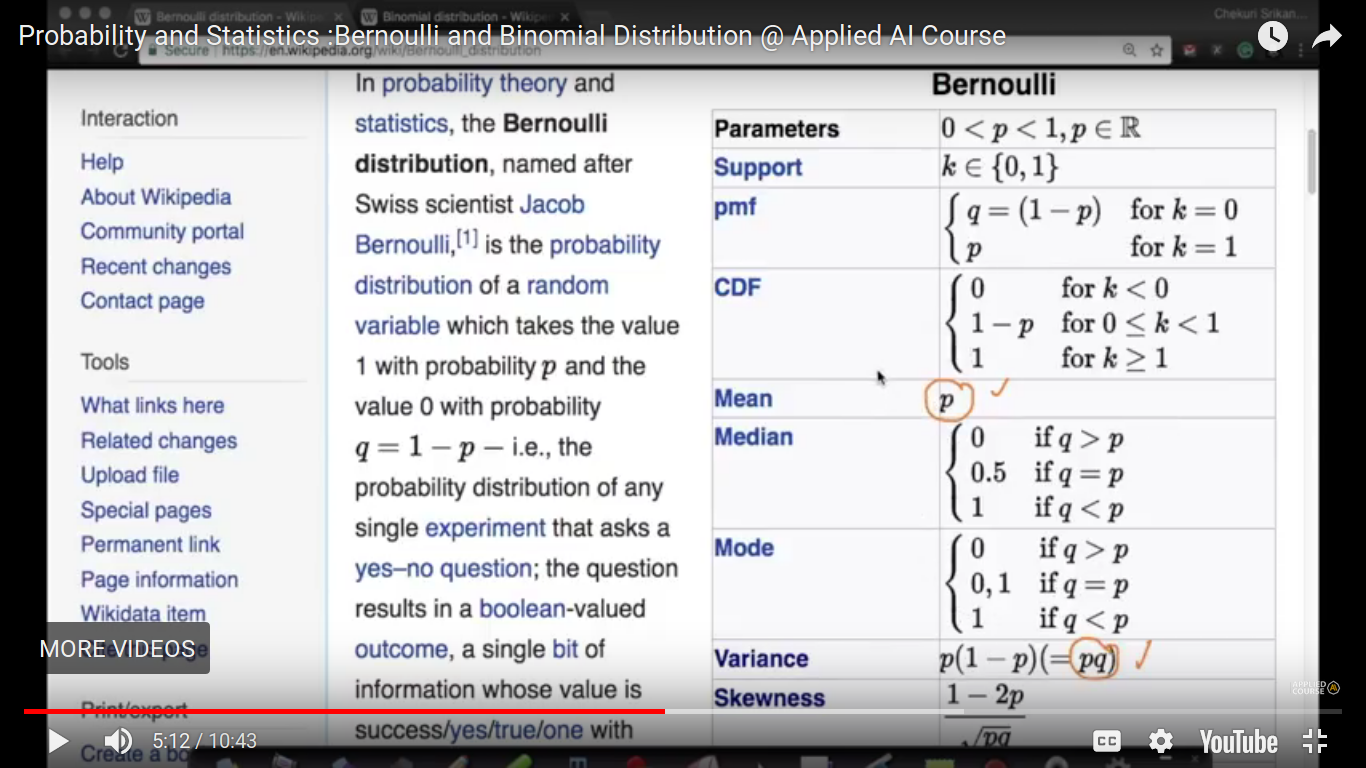
Bernoulli and Binomial Distribution
Bernoulli distribution is the distribution which has literally two outcomes. Example - coin toss
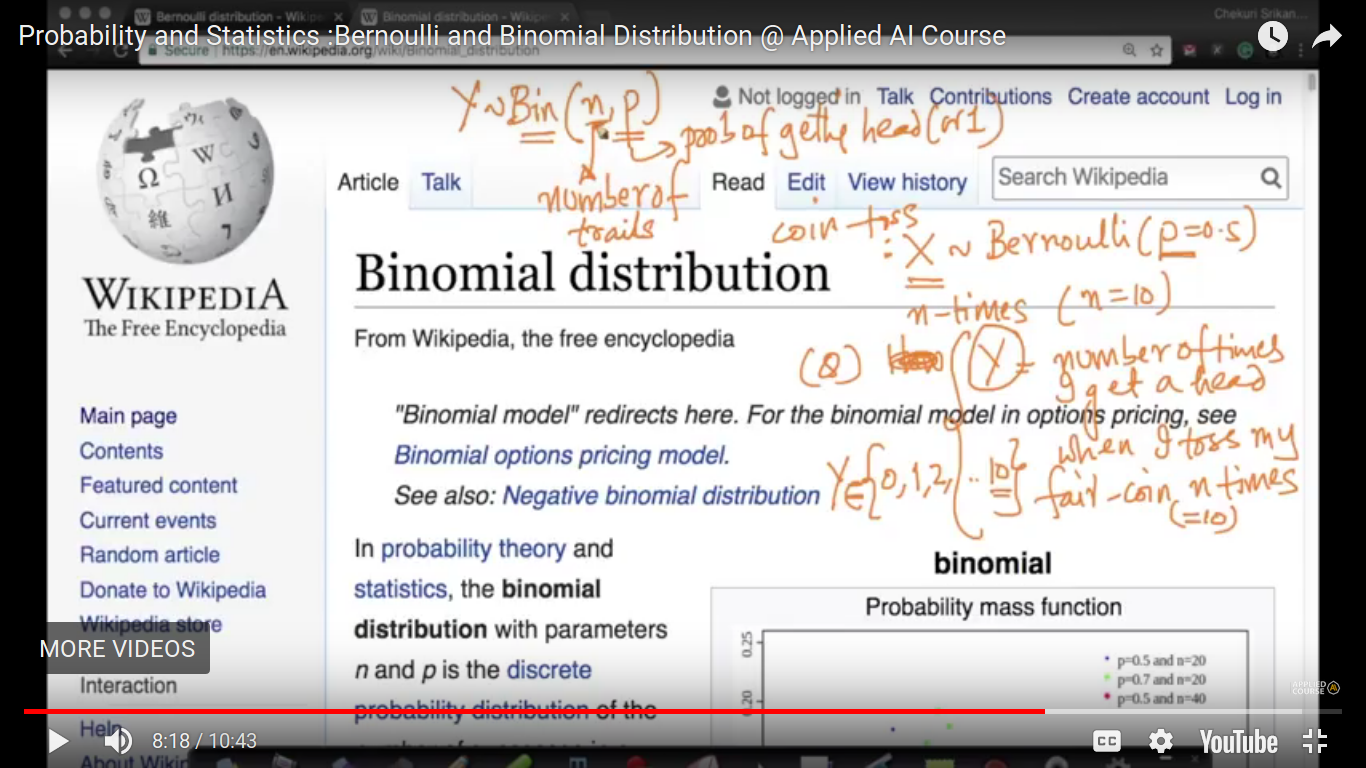
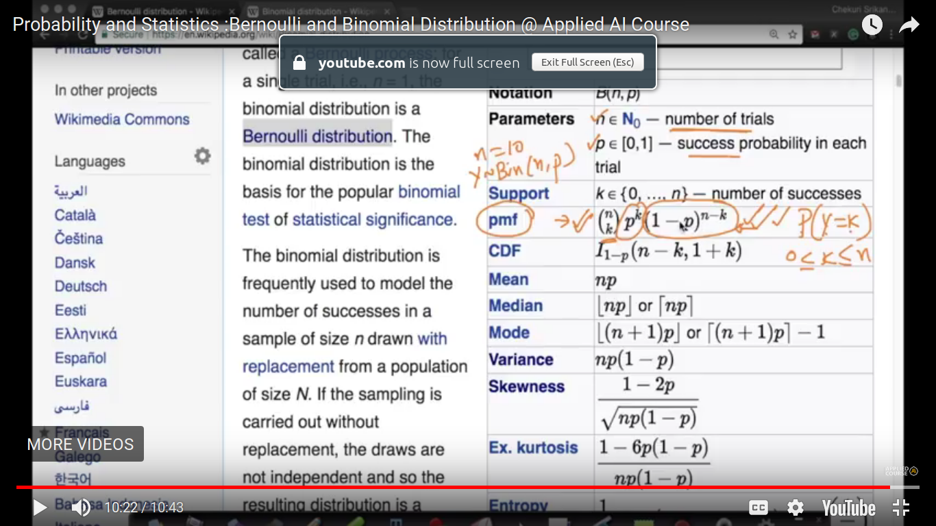
Binomial Distribution -
Page 12
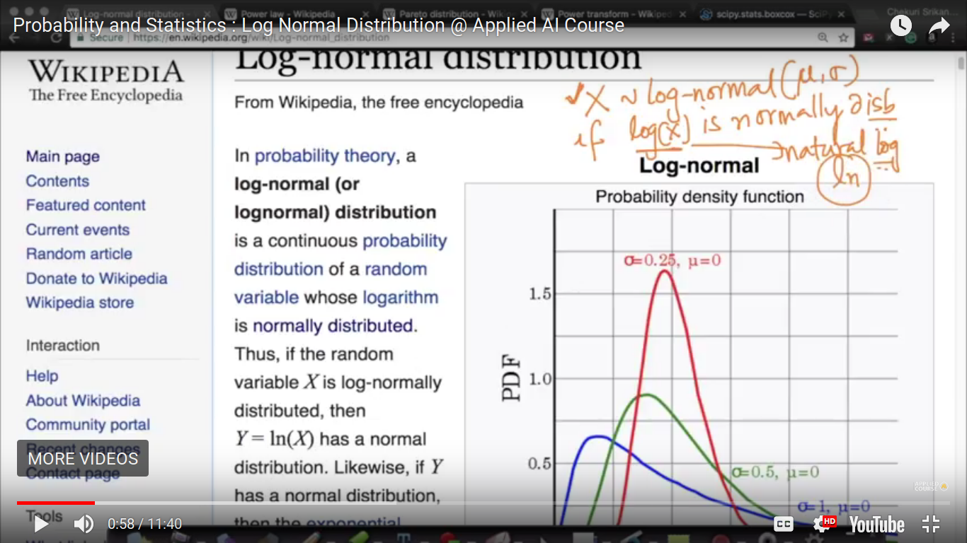
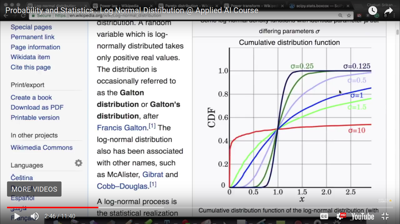
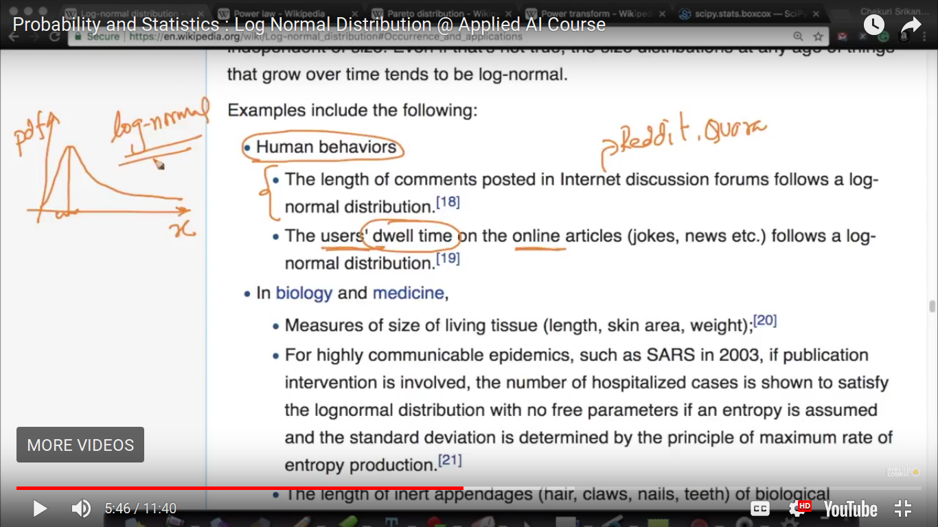
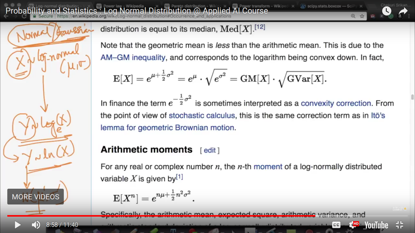
Log Normal Distribution
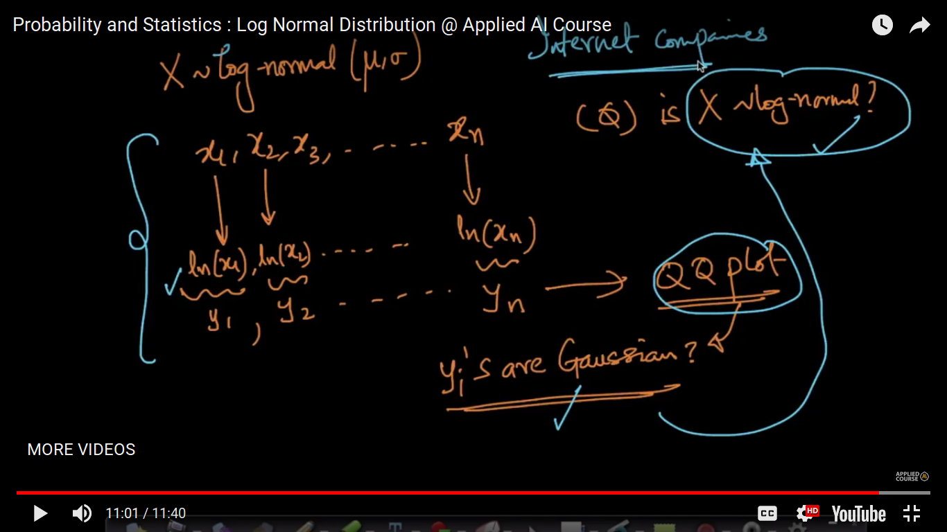
from the logNormal distribution, we can find out it would be normally/Gaussian distributed or not? And further can interpret everything mathematically.
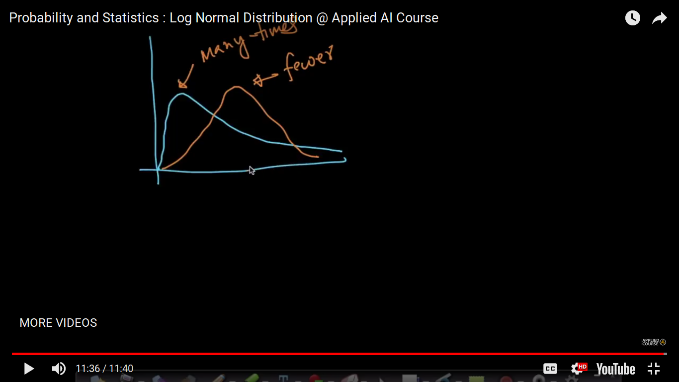
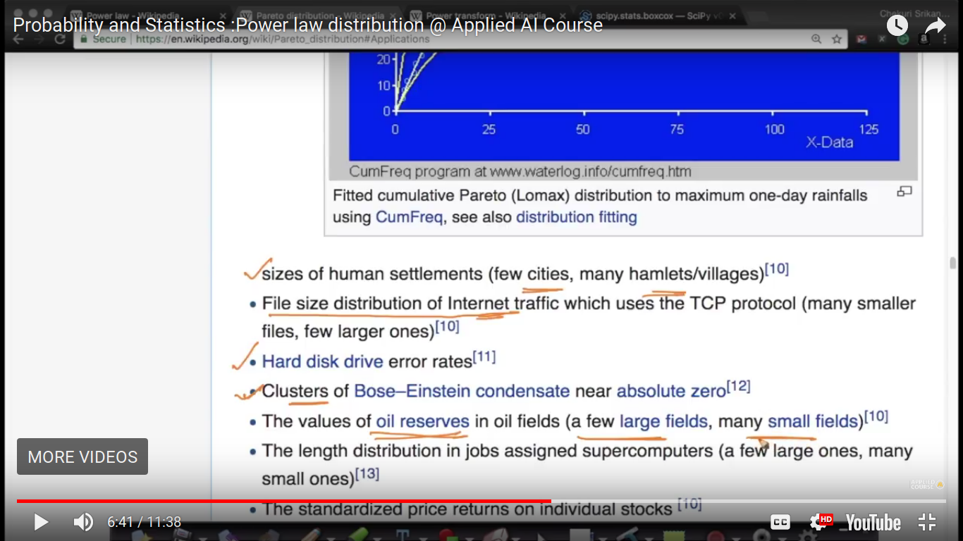
Generally, In Internet-based companies, we can find out many times log-normal or Pareto distribution than others.
Page 13
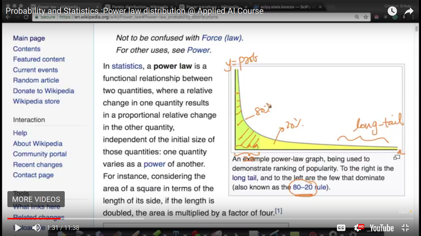
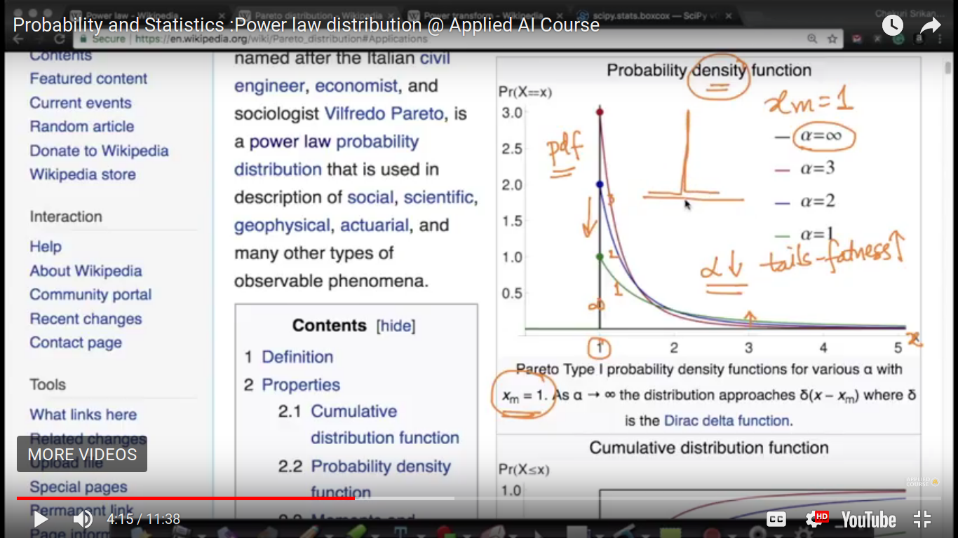
Power Law Distribution
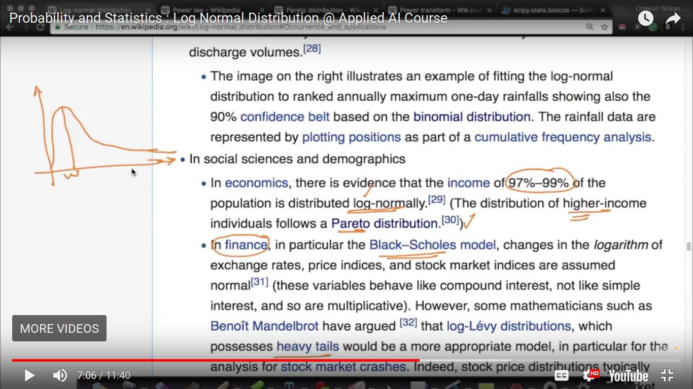
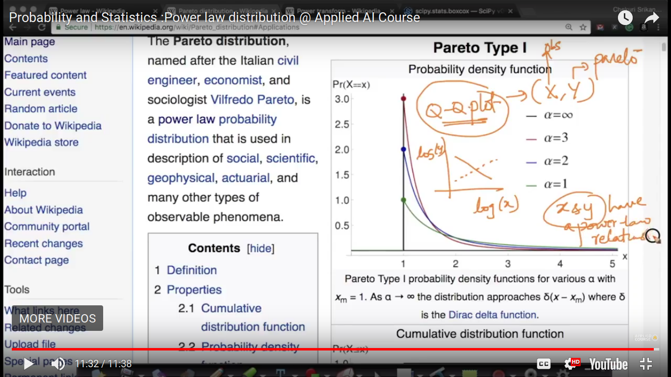
If X follows power law distribution, then it's called Pareto distribution
Dirac Delta Function - Everywhere else is zero but at one given value x=1, it attains peak. When alpha tending to infinity then Dirac delta function condition occurs. So, for Log Normal, it attains a peak value and then a fall off and for Perito distribution, it has a peak value and then slightly fall off.
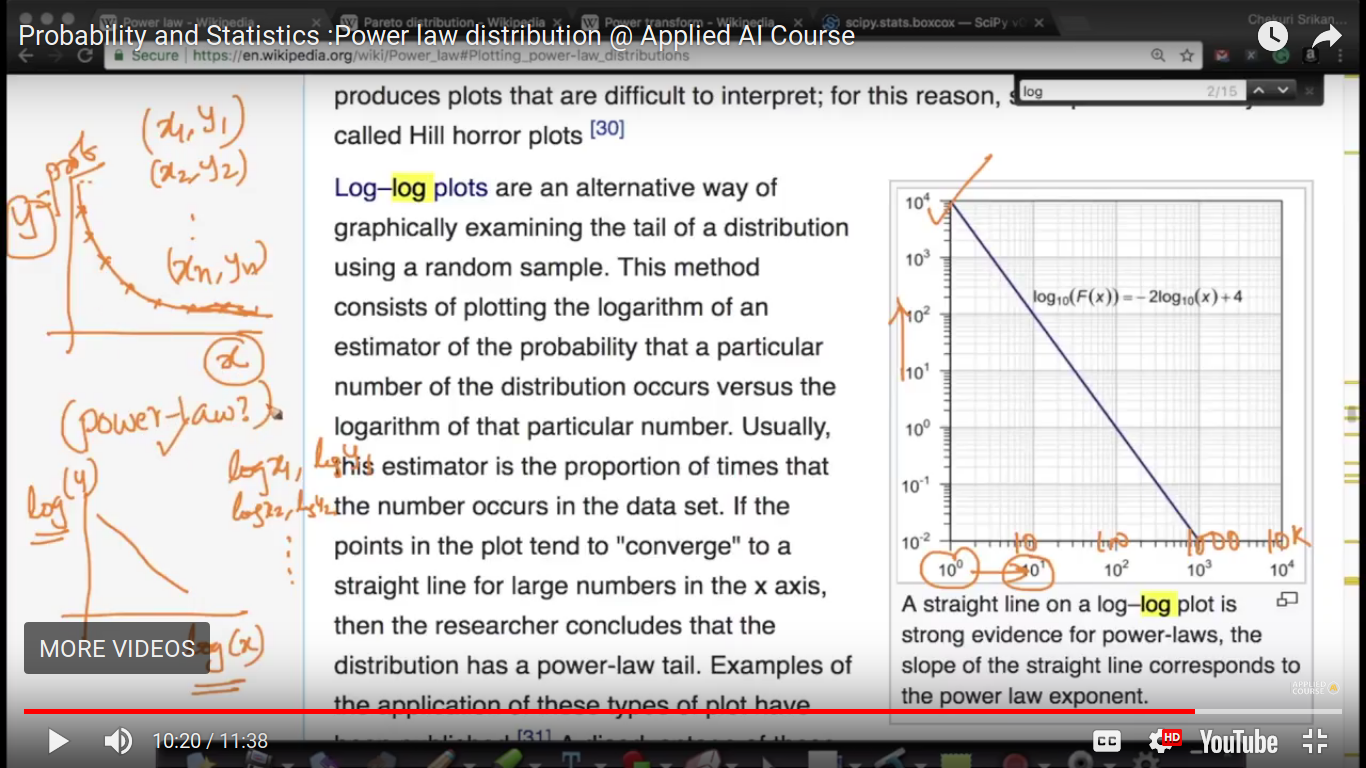
To predict X and Y have a power law relation, we can first find logX and logY and the draw Q-Q plot.
Page 14
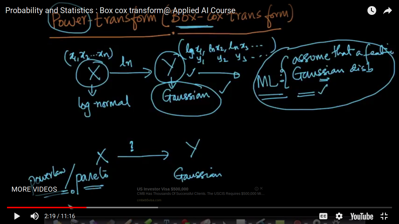
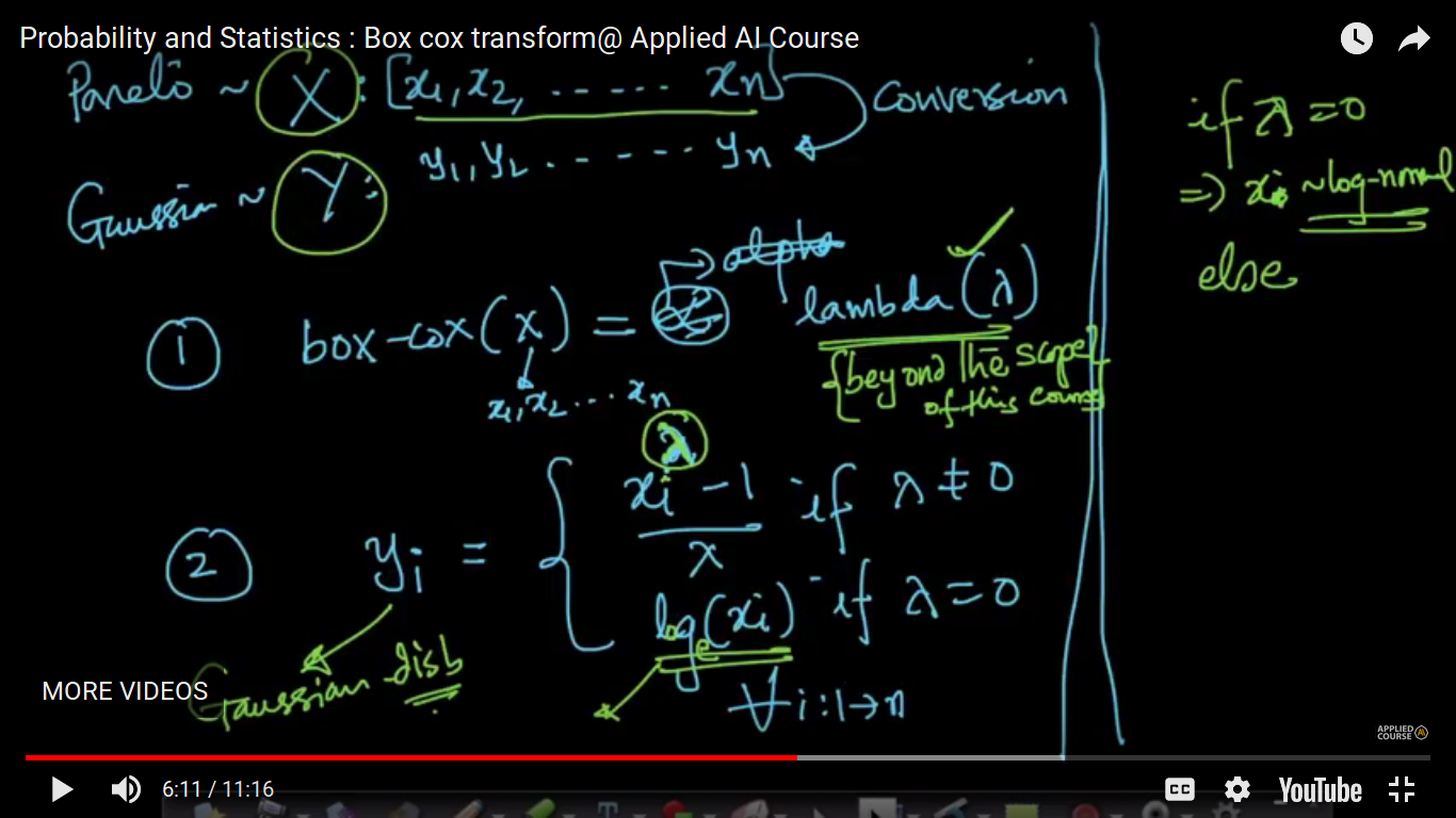
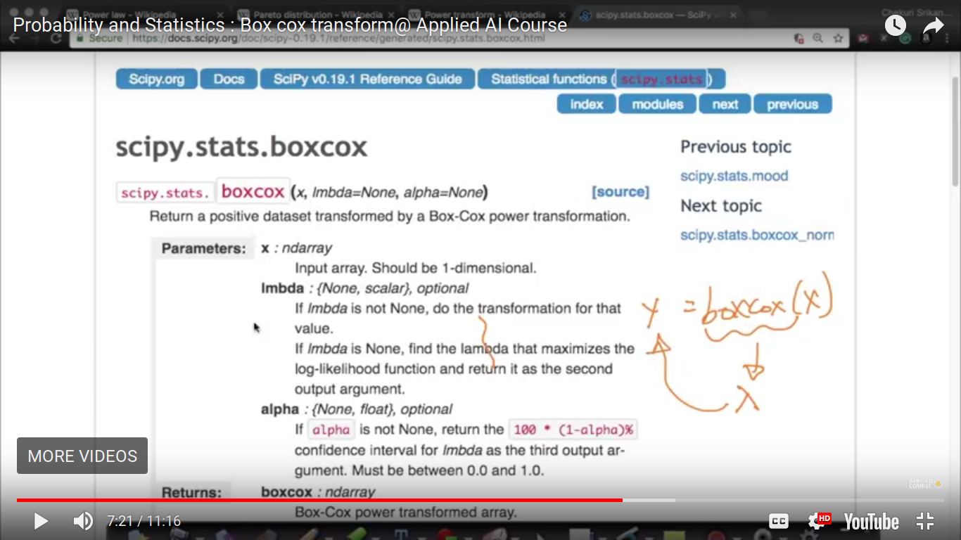
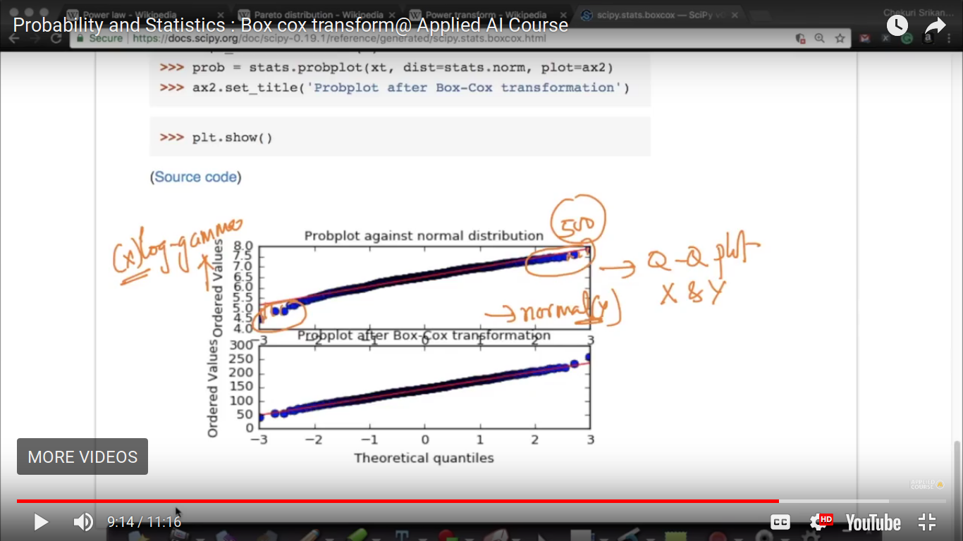
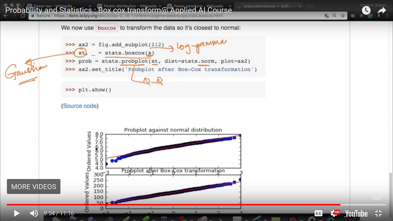
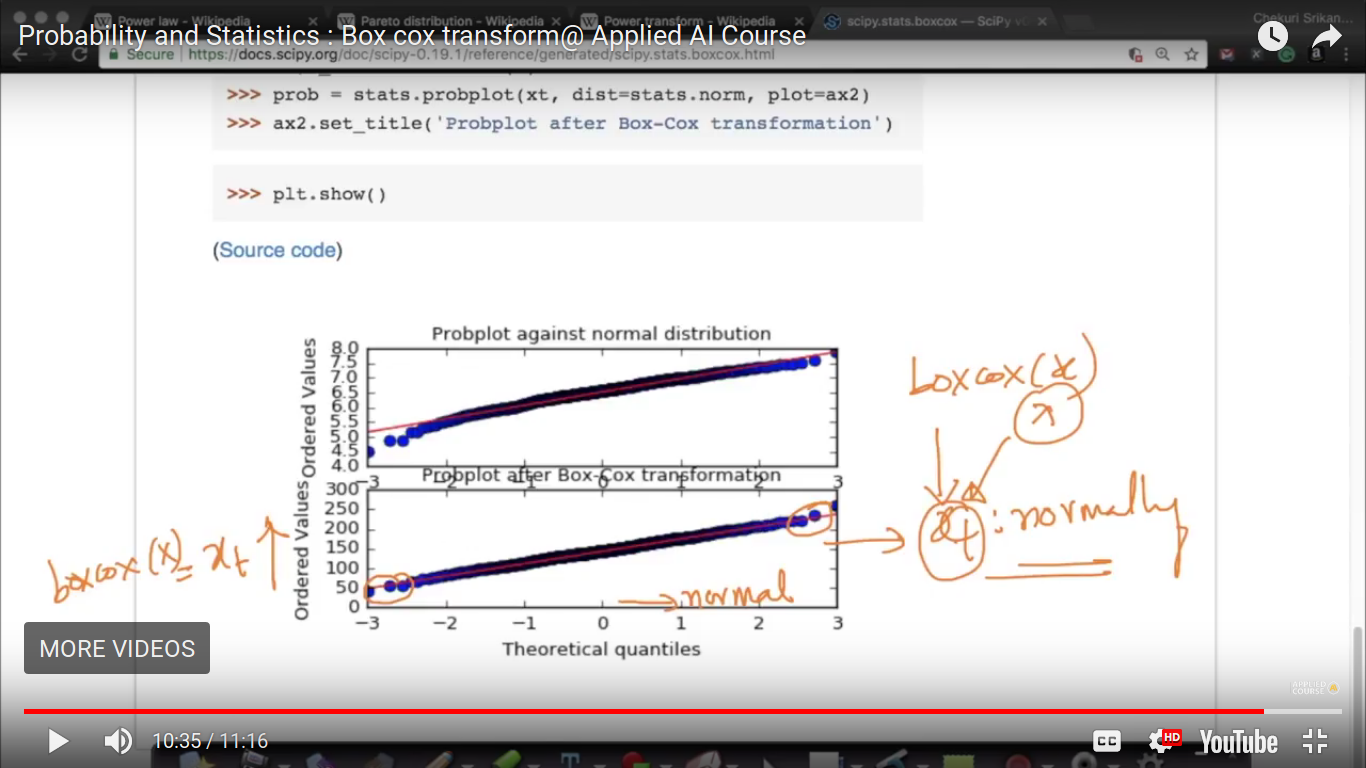
Power Transform (Box-Cox transform)
Here, to transform power Law or Pareto random variable to Gaussian, we are using Power Transform.
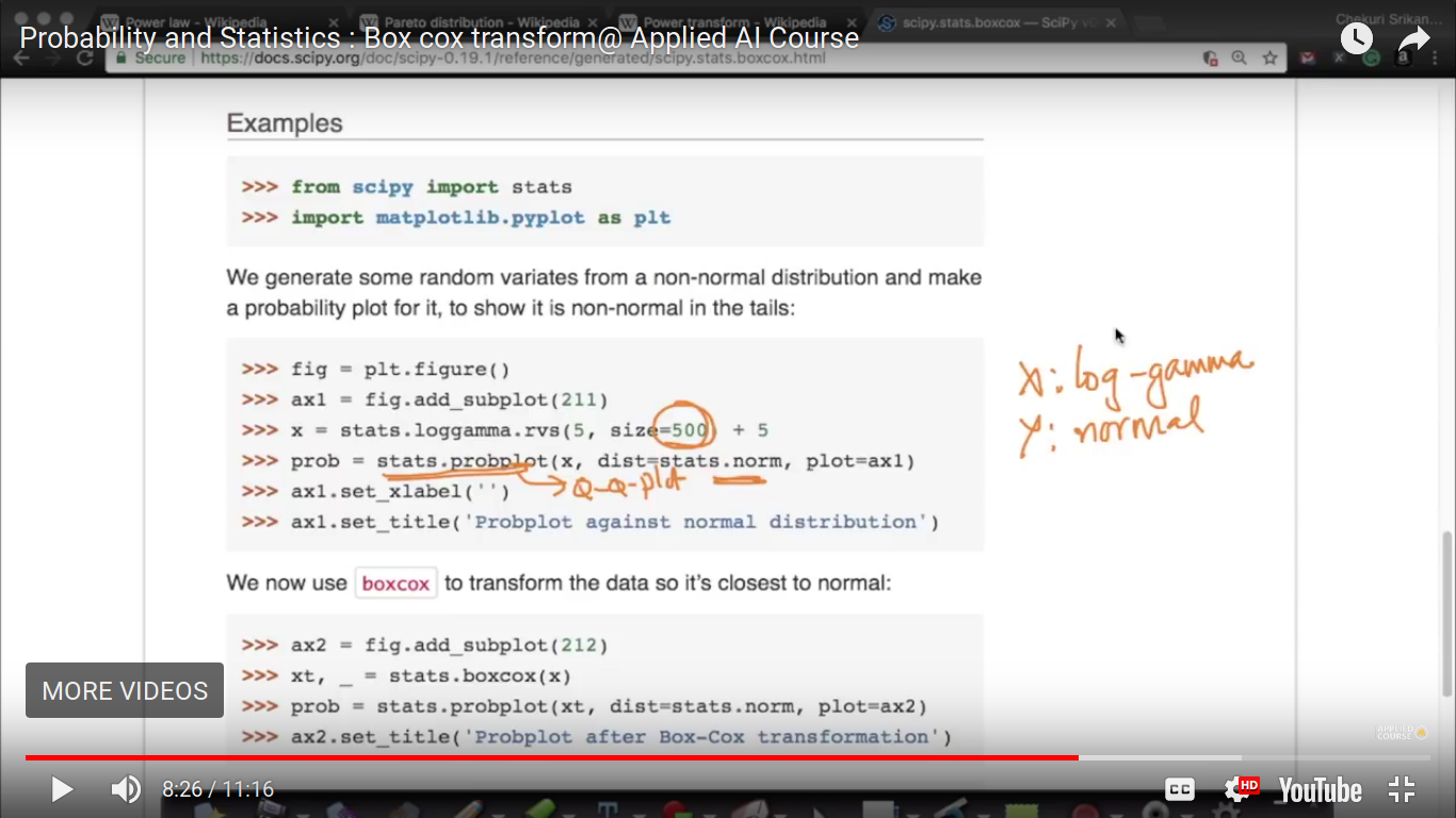
log gamma is not extensively used in machine learning but here it is taken as an example. And log gamma is a Pareto or power law distribution.
Here, there is a significant deviation in the Q-Q plot. So, it means X and Y they belong to the different distribution.
So, now xt is normally distributed. And we found all the extreme points on the straight line which shows they follow a normal distribution.
Page 15
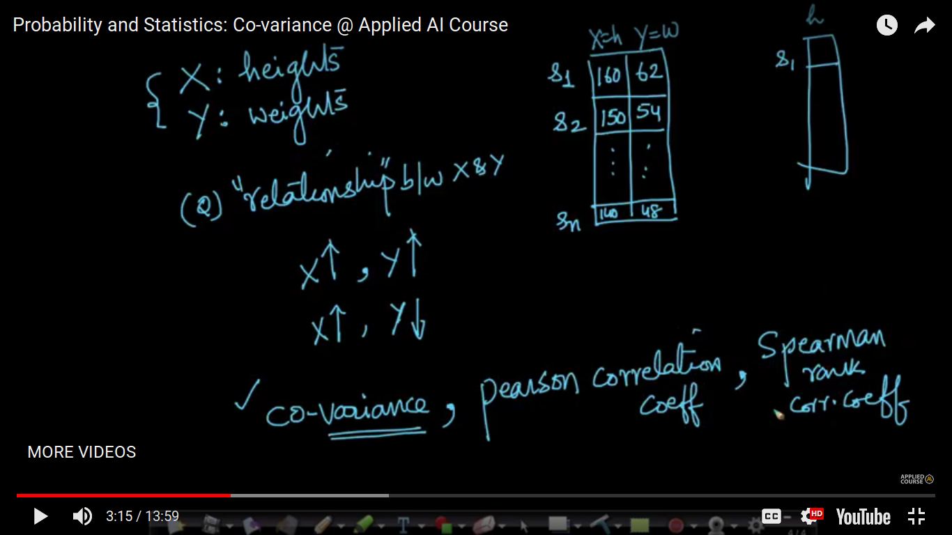
Co-variance
How to measure the relationship between the random variable.
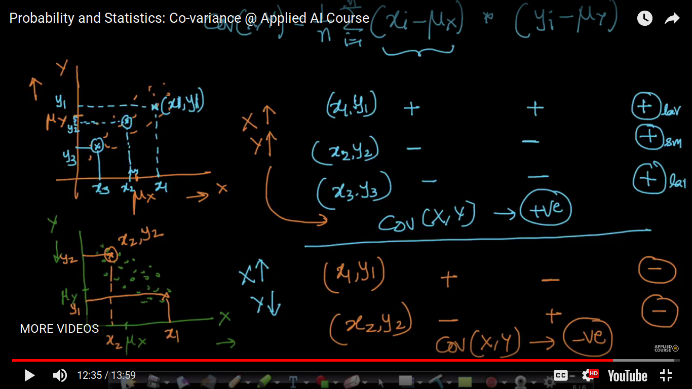
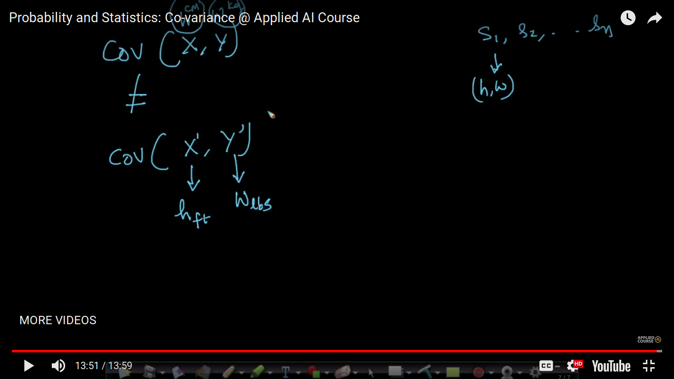
Here, the drawback of Co-variance is that if we change the parameters units. Example cm to fr or kg to lbs, it's covariance not equal. So, further, it's been corrected by Pearson Correlation Coefficient.
Page 16
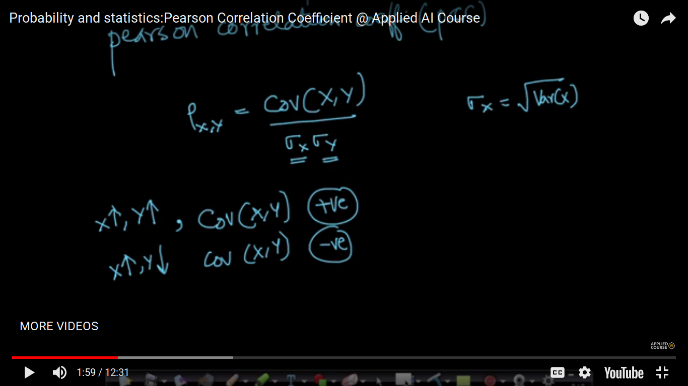
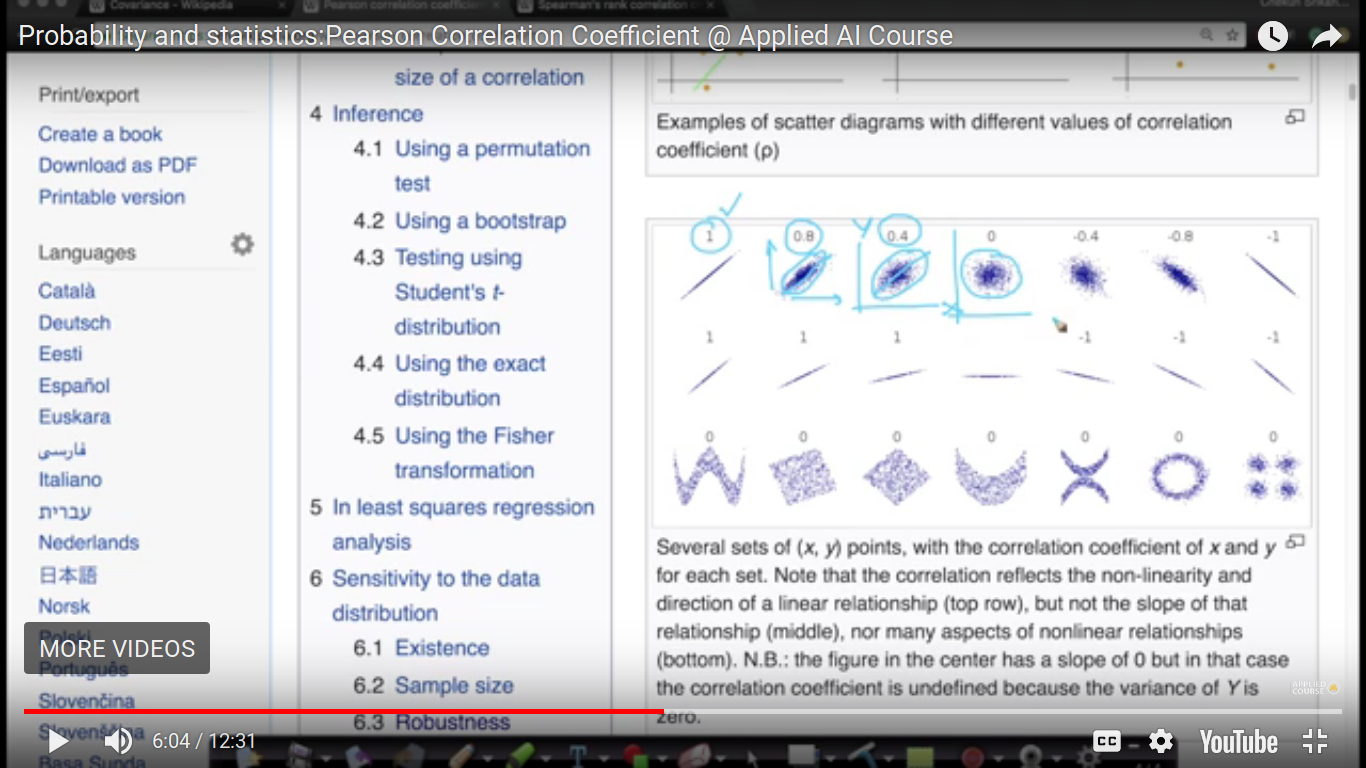
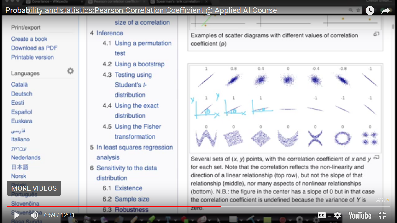
Pearson Correlation Coefficient(PCC)
Another way of measuring the relationship between two random variables. So, the problem with covariance is that it doesn't measure the variability of the variables which is identified in PCC using sigma(x) and sigma(y) i.e standard and deviations. For Example - We know if x increases and then y also increases, it means Covariance becomes +ve but we don't how much it's positive i.e don't know about its variability. PCC=0 or rho=0 means no relationship between X and Y. https://www.goconqr.com/en/notes/14442551/edit
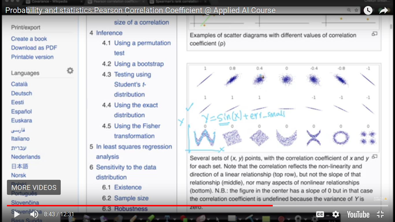
Slope doesn't matter in case of PCC. PCC cannot capture complex non-linear relationships i.e it doesn't find relationships. So, its value is zero. And we are building a full-fledged model like the regression model.
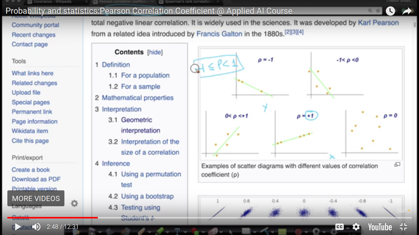
And if Y2>Y1, then it is called monotonically increasing. The above relationship seems to be no-linear and we are gonna fix it using our next topic.
Page 17
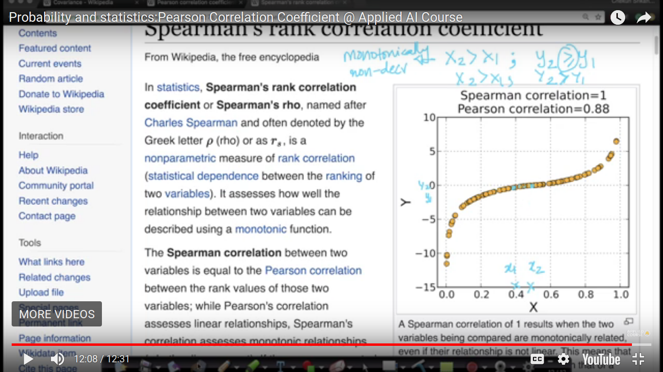
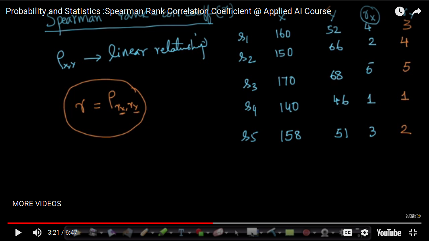
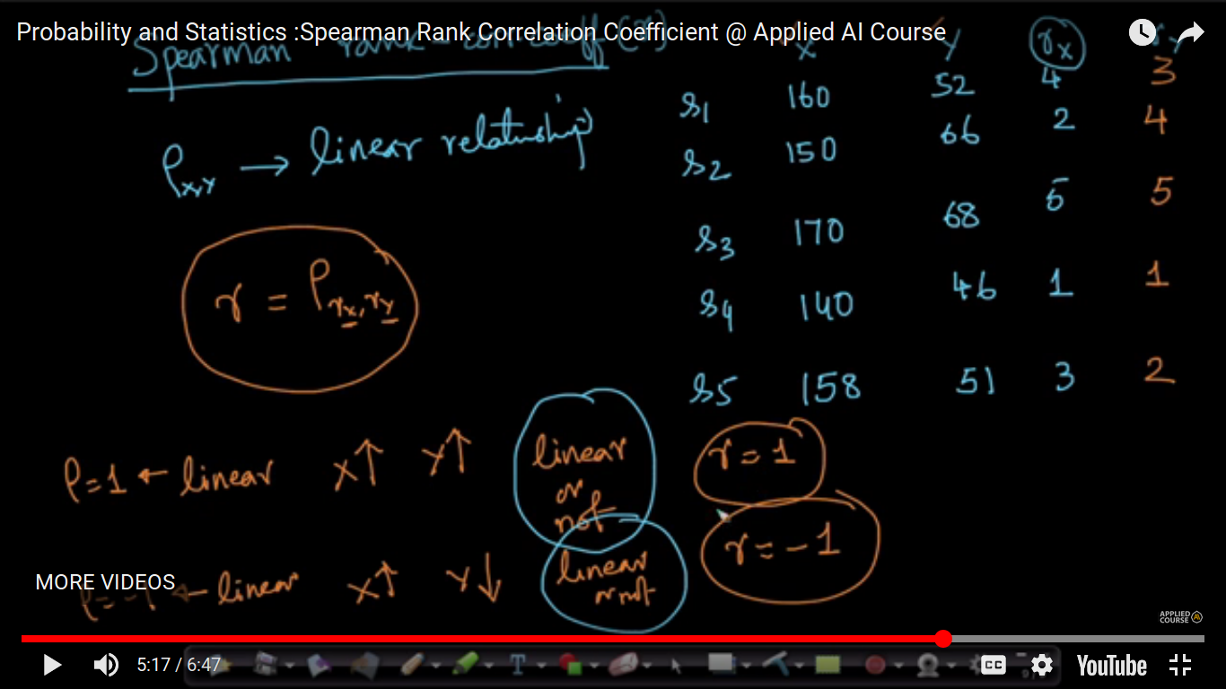
Spearman Rank Correlation Coefficient
PCC method is valid for linear relationships only. So, this method will not fix a complex relationship but it will resolve monotonically non-decreasing relationships.
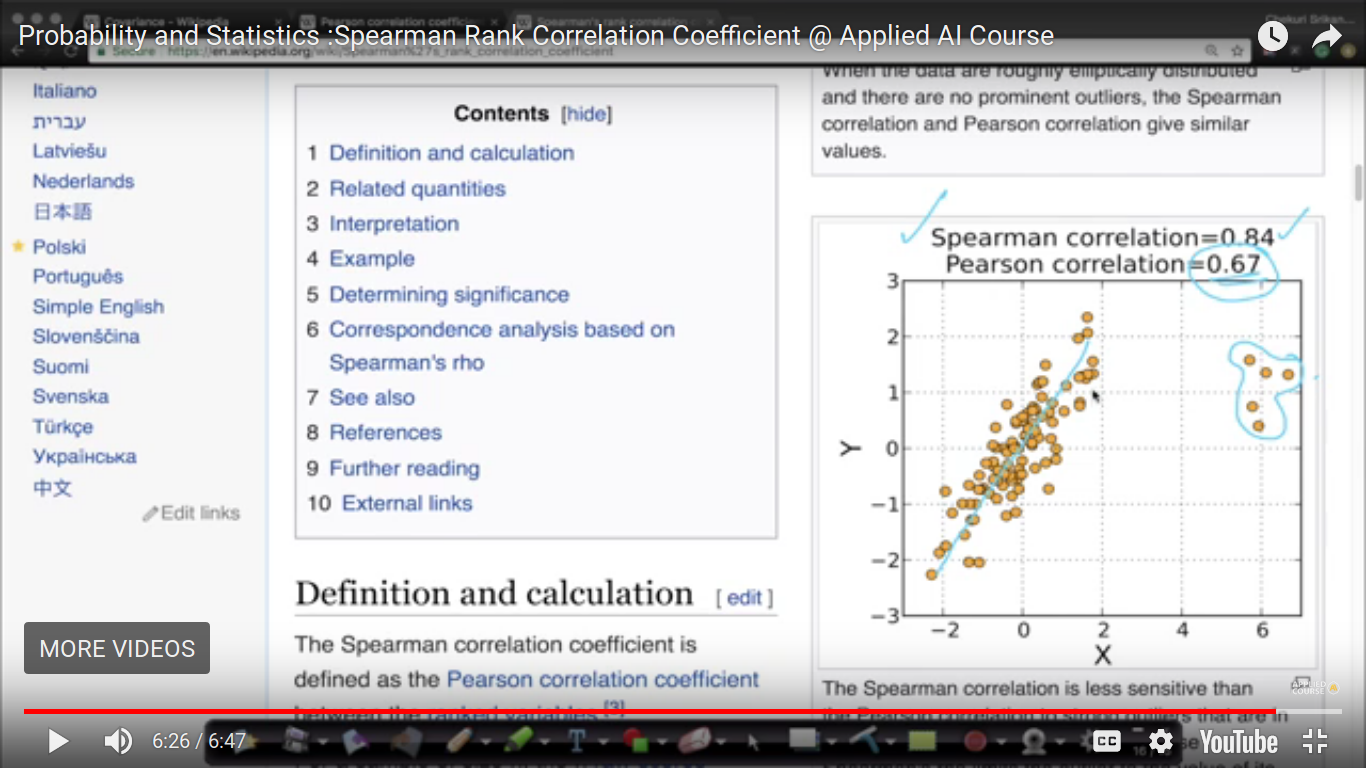
Spearman relationship is nothing but the Pearson Coefficient of the rank of X and Y
Page 18
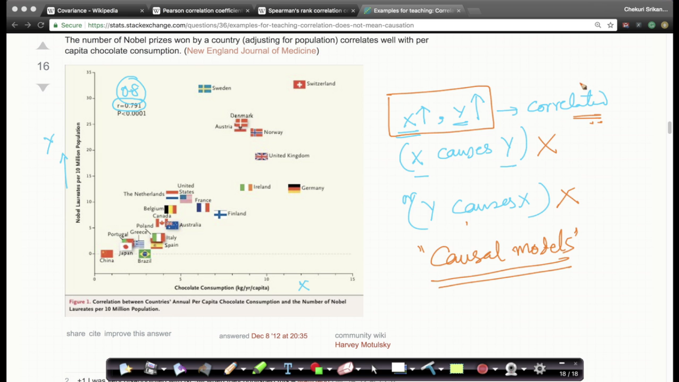
Correlation vs Causation
If X and Y are co-related then it is absurd to say that the X causes Y i.e it doesn't mean X causes Y
Page 19
Confidence interval (C.I) Introduction
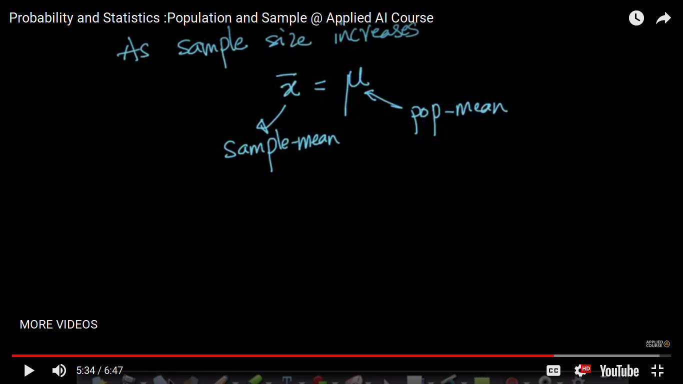
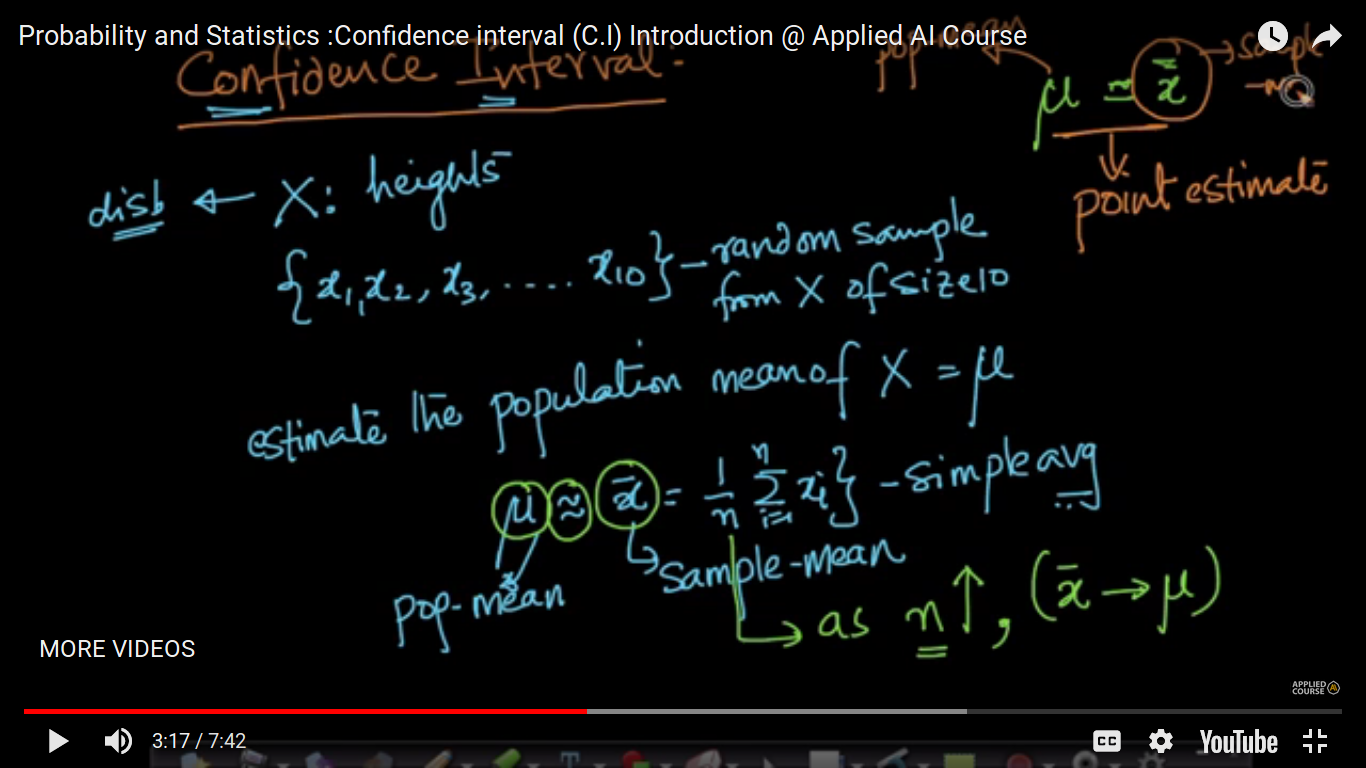
Point Estimate - It means we are just finding the sample mean of some random values which may be equal to the population mean. So, we find another way to do the same and its called Confidence Interval. Here, As n increases xbar closer to mu.
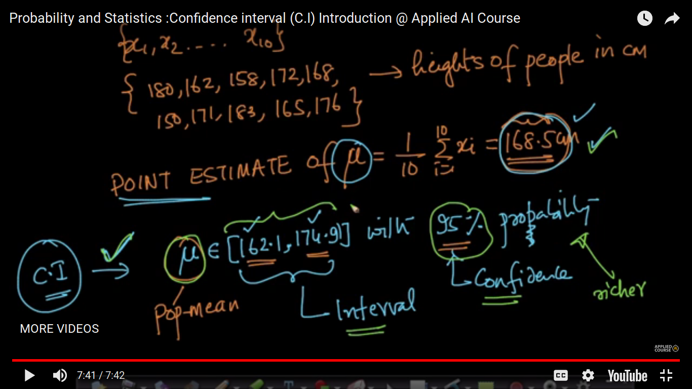
So, C.I. is richer in Information. It defines internal with the appropriate probability.
Page 20
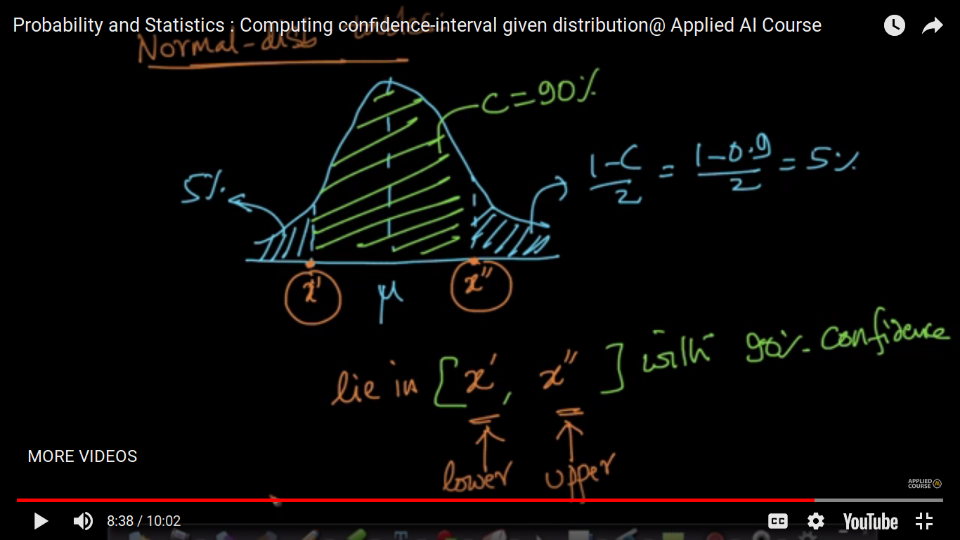
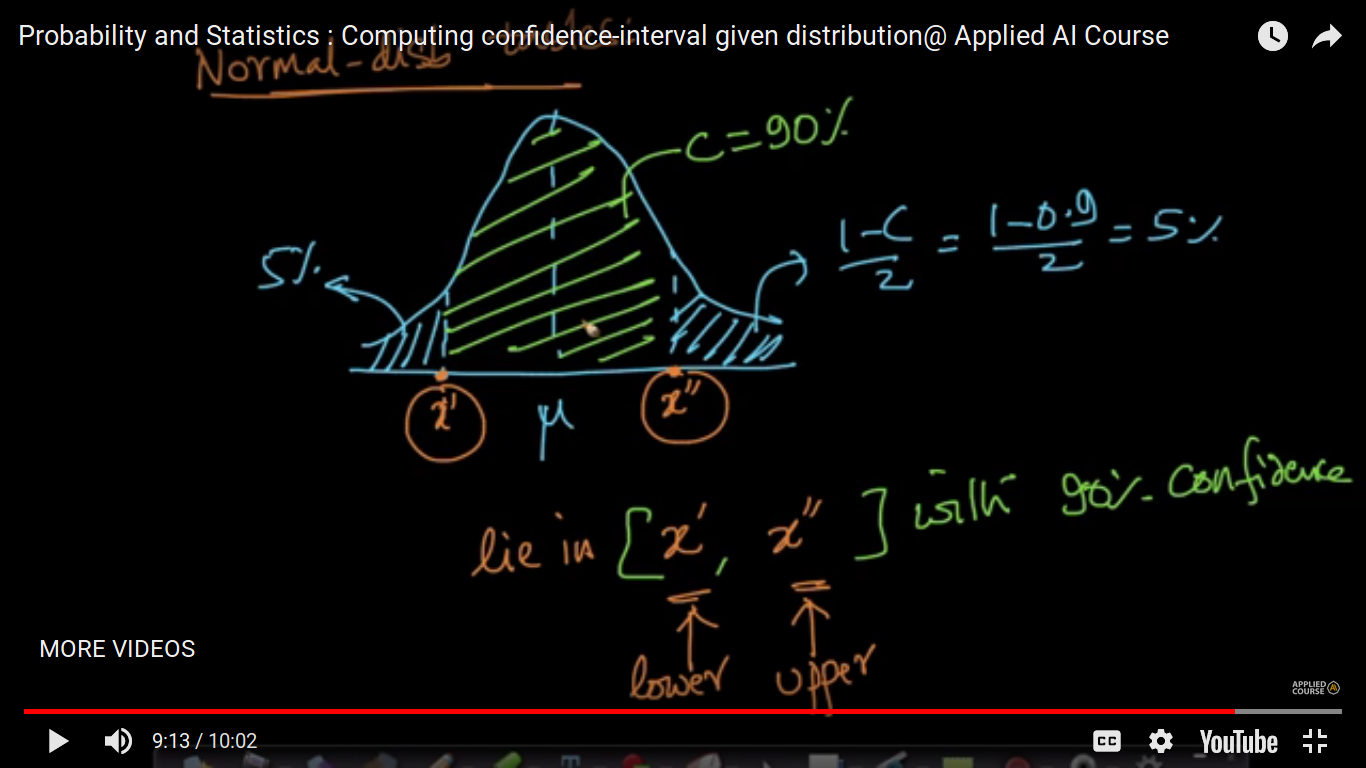
Computing confidence interval given the underlying distribution
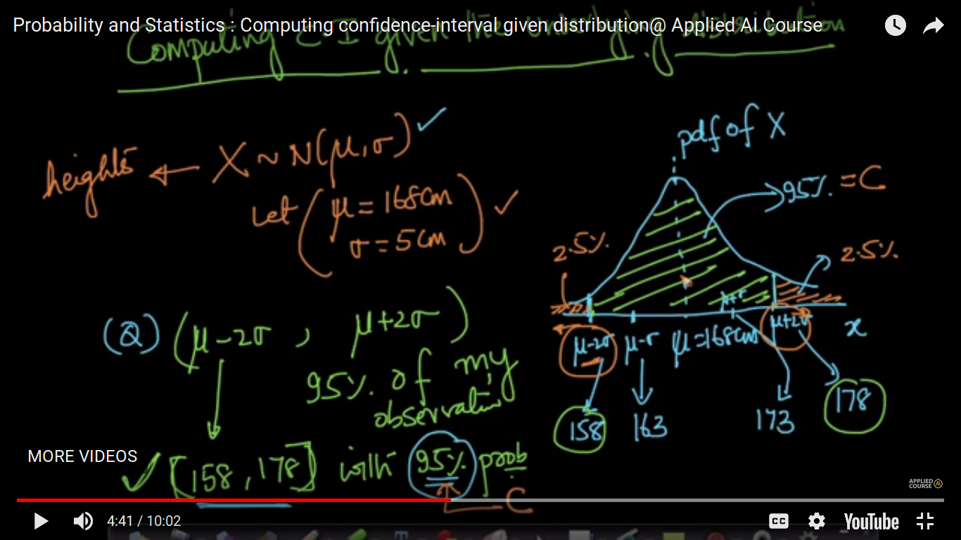
Here, we assume X follows the Normal or Gaussian distribution.
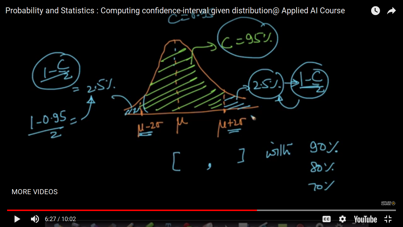
If we are talking about calculating the value of x' and x'' for 90 percent, we have to use the Normal distribution table because if X follows the Normal distribution, then we always talk about 95 percent data which is easily calculatable using variance and mean but for calculating another percentage, we have to use a table.
Page 21
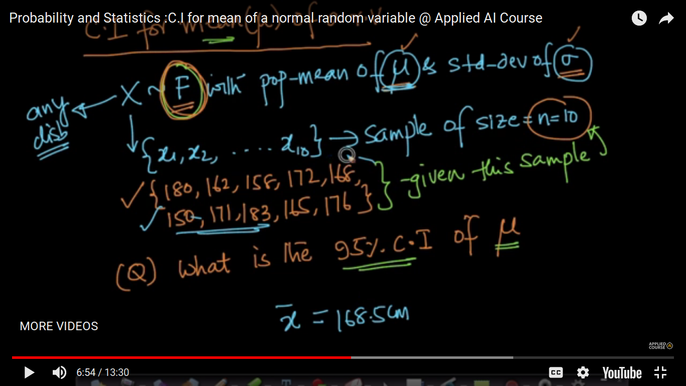
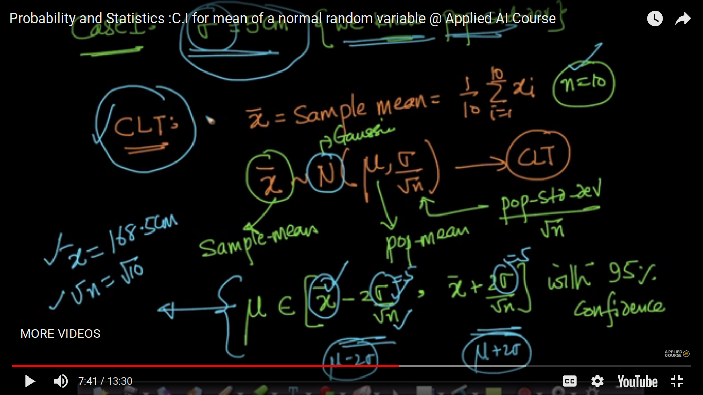
C.I for mean of a normal random variable
CLT - Central limit theorem
We can find out 95 percent CI of the mean for any distribution.
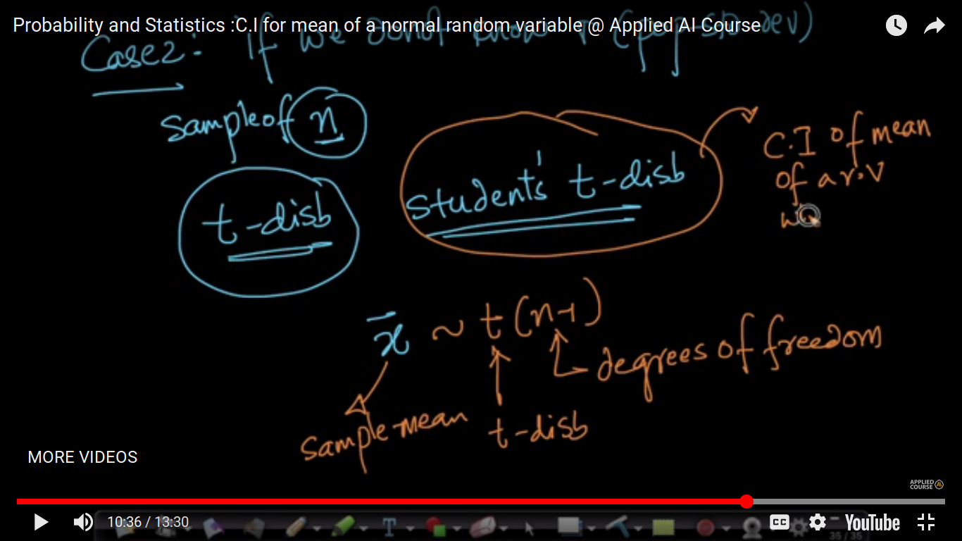
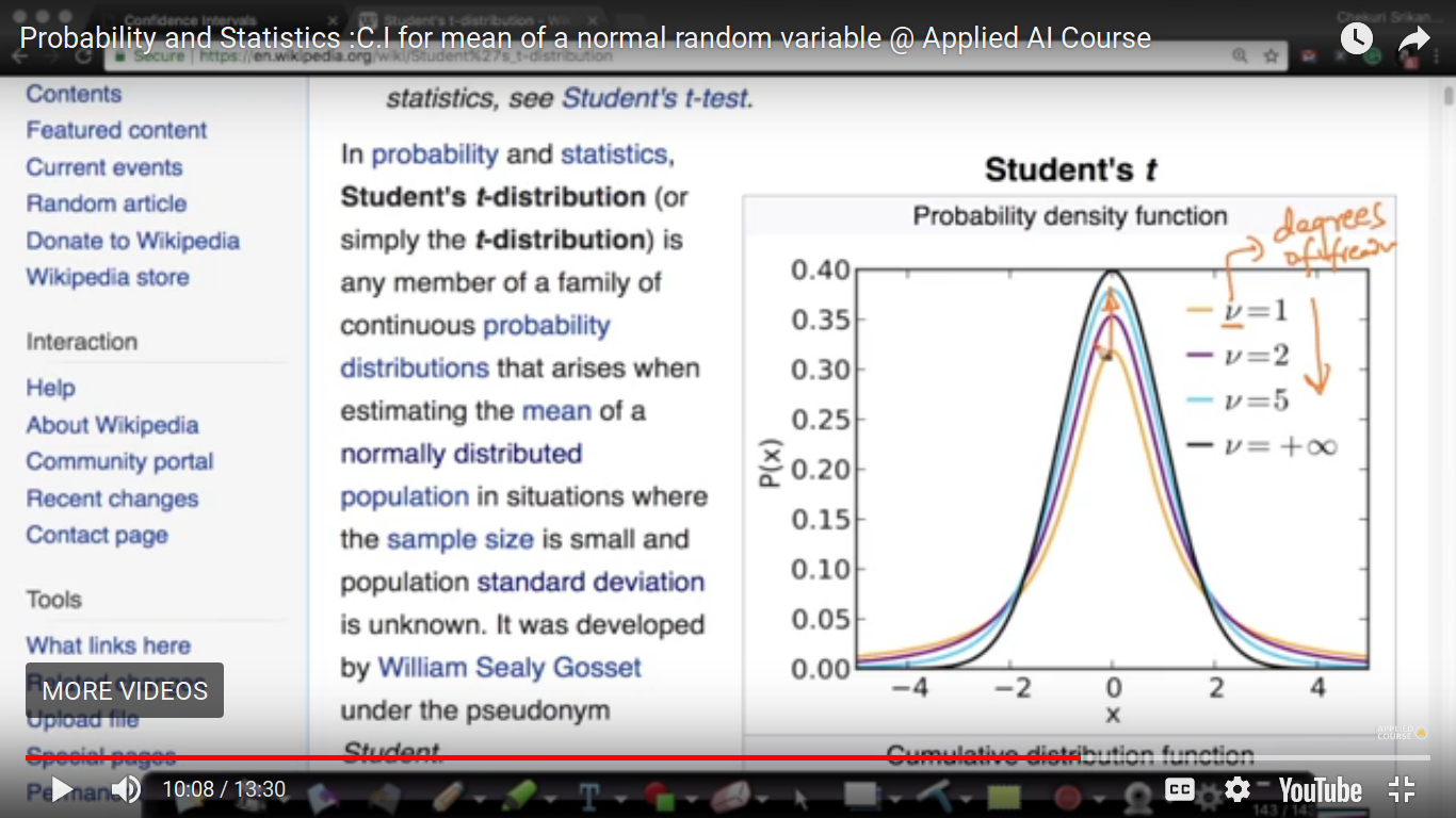
Students t-distribution - One of the biggest application of this is to compute the confidence interval for the mean of a random variable when the standard deviation is not given.
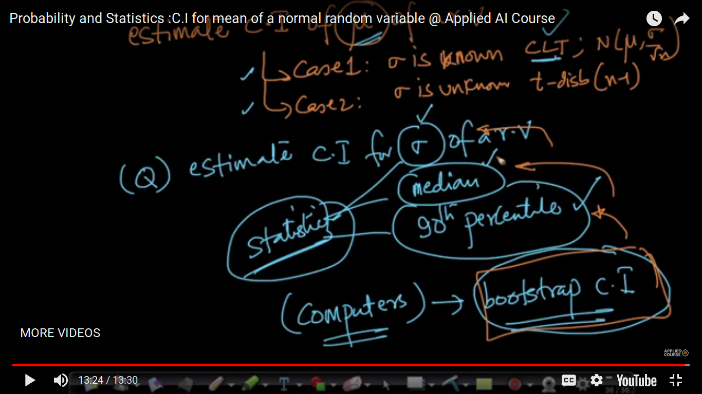
The above two cases - Case 1: Sigma is known where CLT and Gaussian distribution. Case 2: Sigma is Unknown where we use t-distribution with (n-1) degree of freedom. So, we can only able to compute CI for the mean of a random variable and not for CI for a median, standard deviation, 90th percentile. So, this will be computed using Bootstrap C.I.
1. If you have too little data like 10 points, the C.I estimate would be very incorrect. You will need a decent amount of data for your C.I to be reasonable. More data, better is your estimate of C.I. 2. Yes, you are correct if we know the population std-dev, sigma as in case 1 in the video. 3. Yes, because from CLT, x_bar follows a gaussian-disb as stated at 3:39 in the video. And, we know that 68% of values lie in 1-std dev range around the mean for gaussian disb. Yes, as N increases, x_bar would tend to mu as expected. 4. IN both cases 1 and 2, we are working off of a sample. We do not have the population. In case 1, we only know population-std-dev and nothing else. If we had the whole population, we can easily compute the mu and why bother about C.I of mu? 5. Here in C.I, we are estimating the 95% of mu using the sample. When we studied distributions, mu and sigma are params of the distribution which are useful for explaining the disb.
Page 22
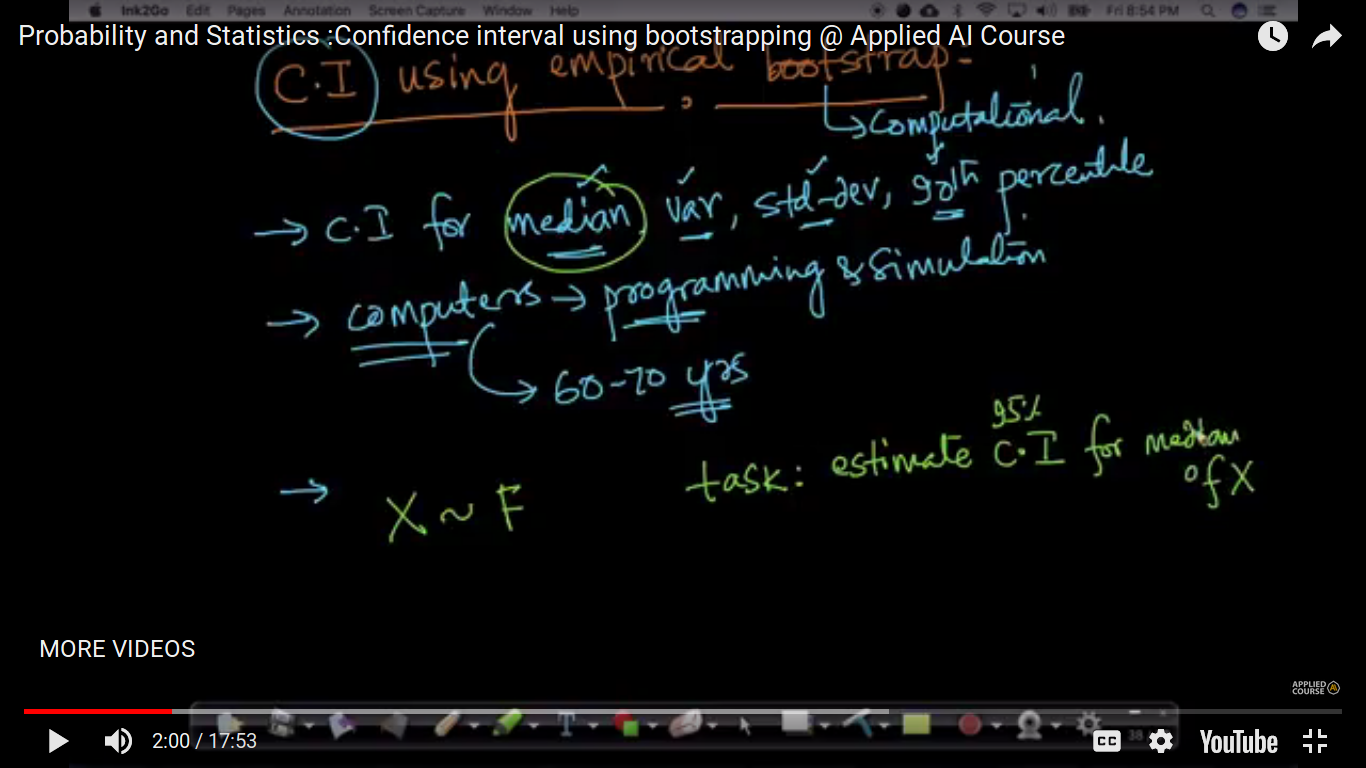
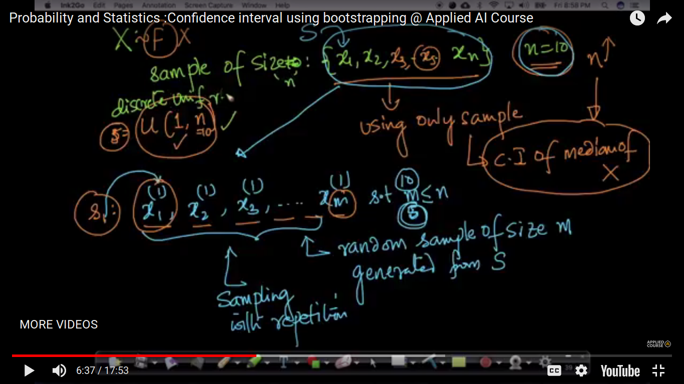
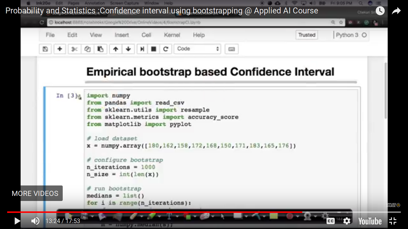
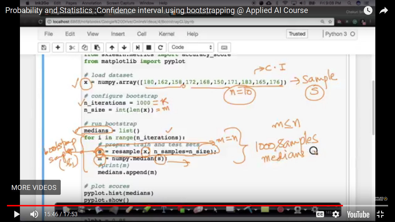
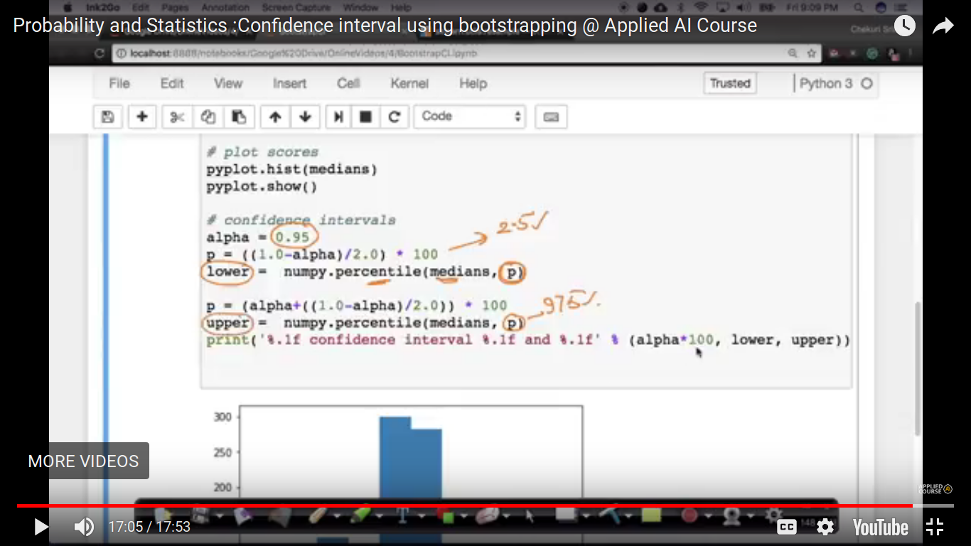
Confidence interval using bootstrapping(Very Imp for CI))
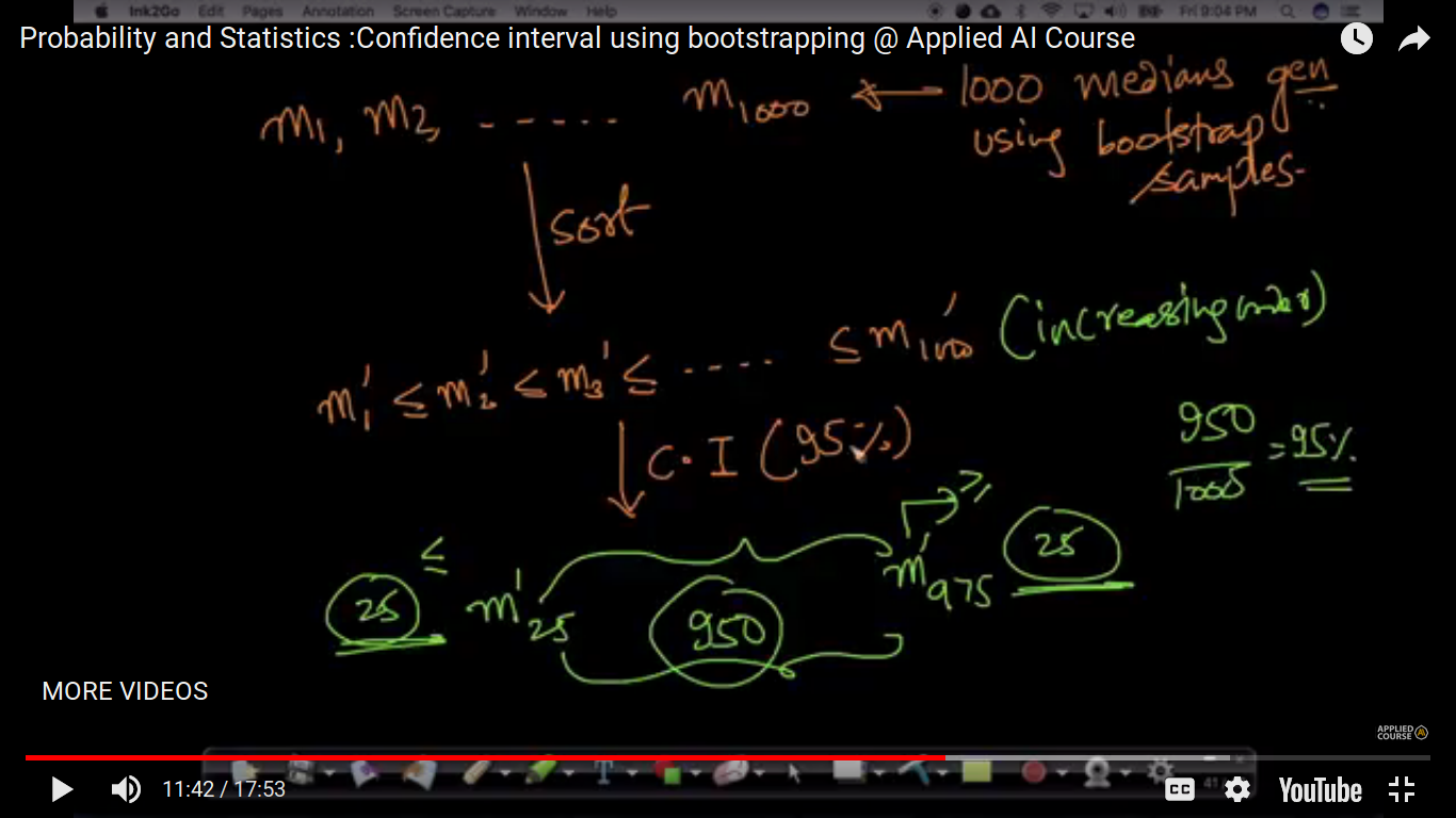
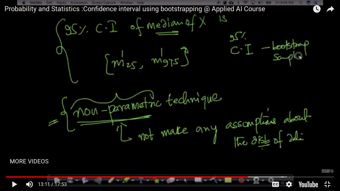
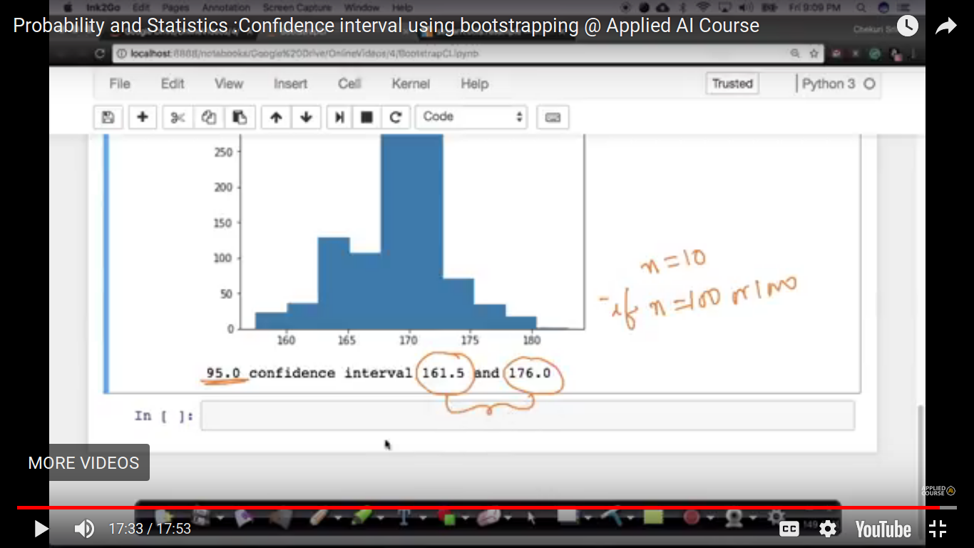
Here, we don't know what kind of distribution we have. We take n as a reasonable value(not so small) i.e preferably take above 20. If n increases, we will be able to estimate C.I. of median better.
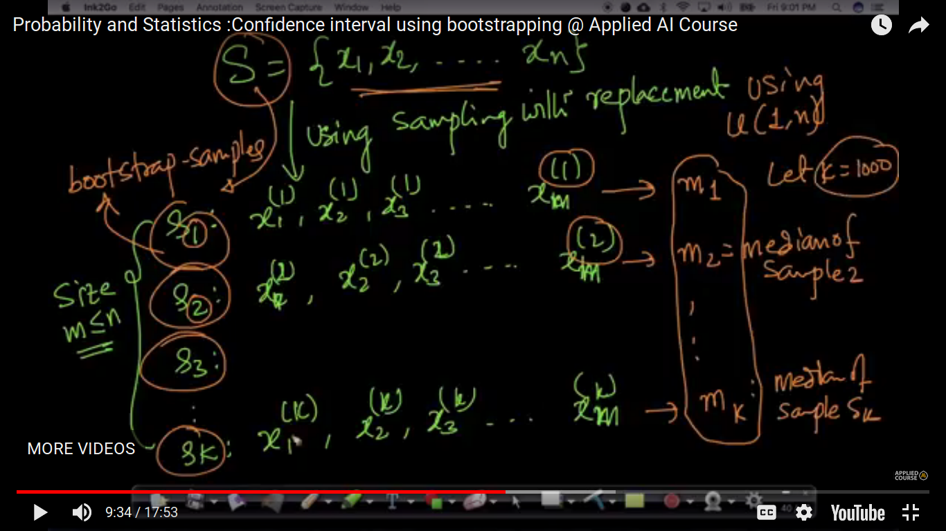
Values in any sample may be repeated in another. We use u(1,n) uniform discrete random variable to generate each of the samples. bootstrap samples are artificially created.
If n is 100 or 1000 instead of 10, the difference of 161 to 176 is closer than that.
Page 23
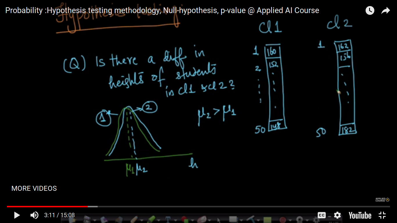
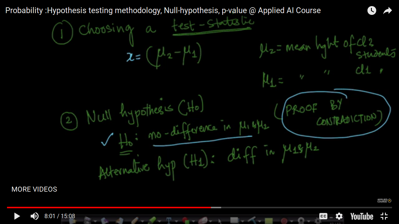
Hypothesis testing methodology, Null-hypothesis, p-value
Page 24
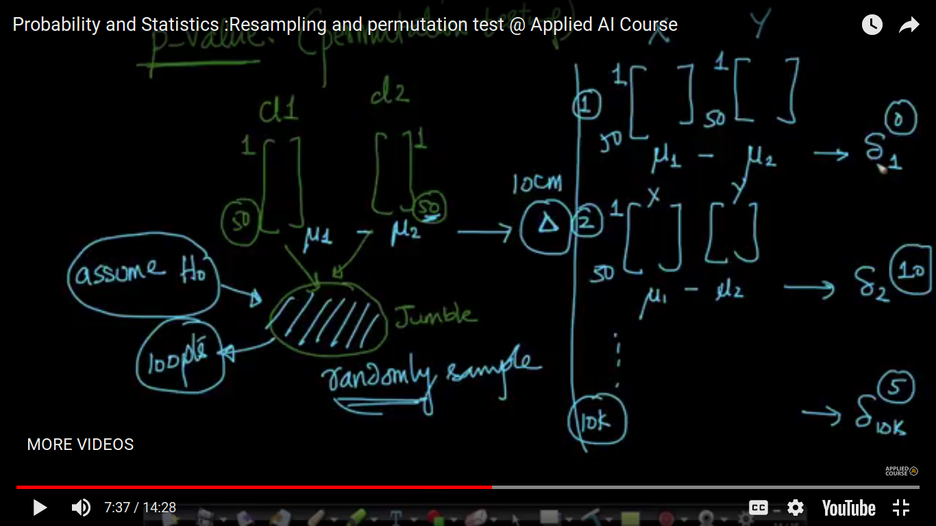
Resampling and permutation test
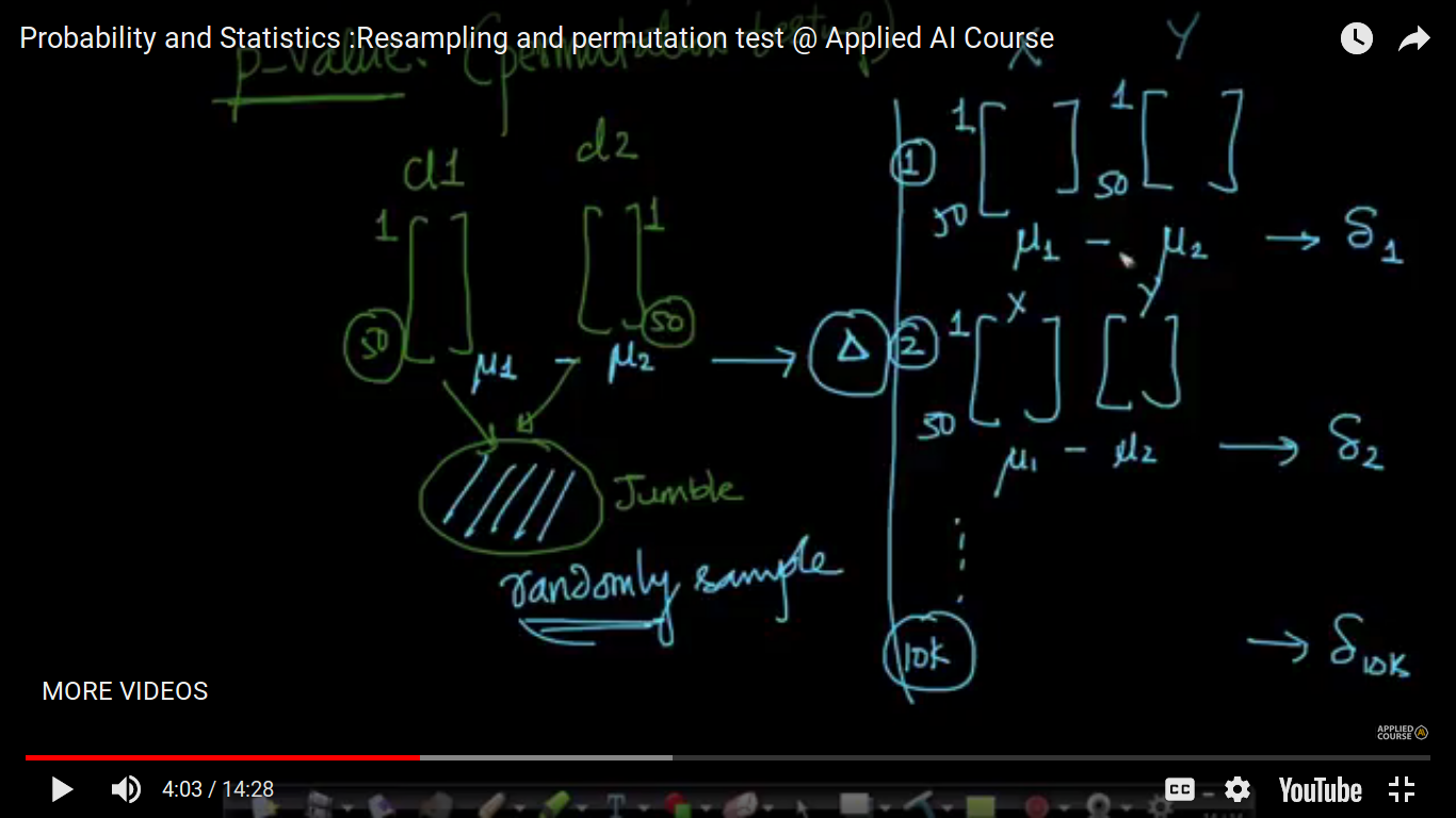
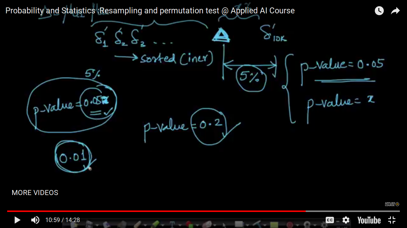
We accept a hypothesis based on the p-value. Interesting idea to compute value is the permutation testing.
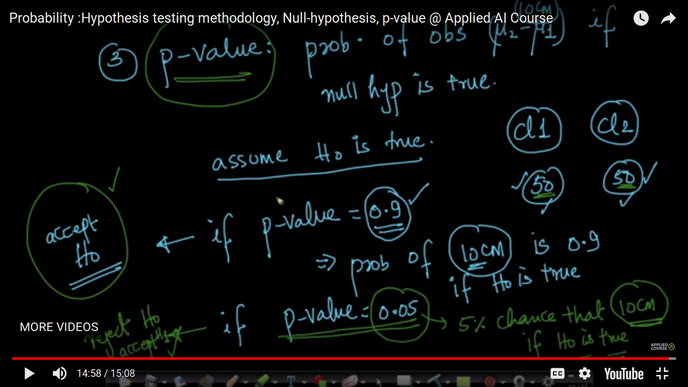
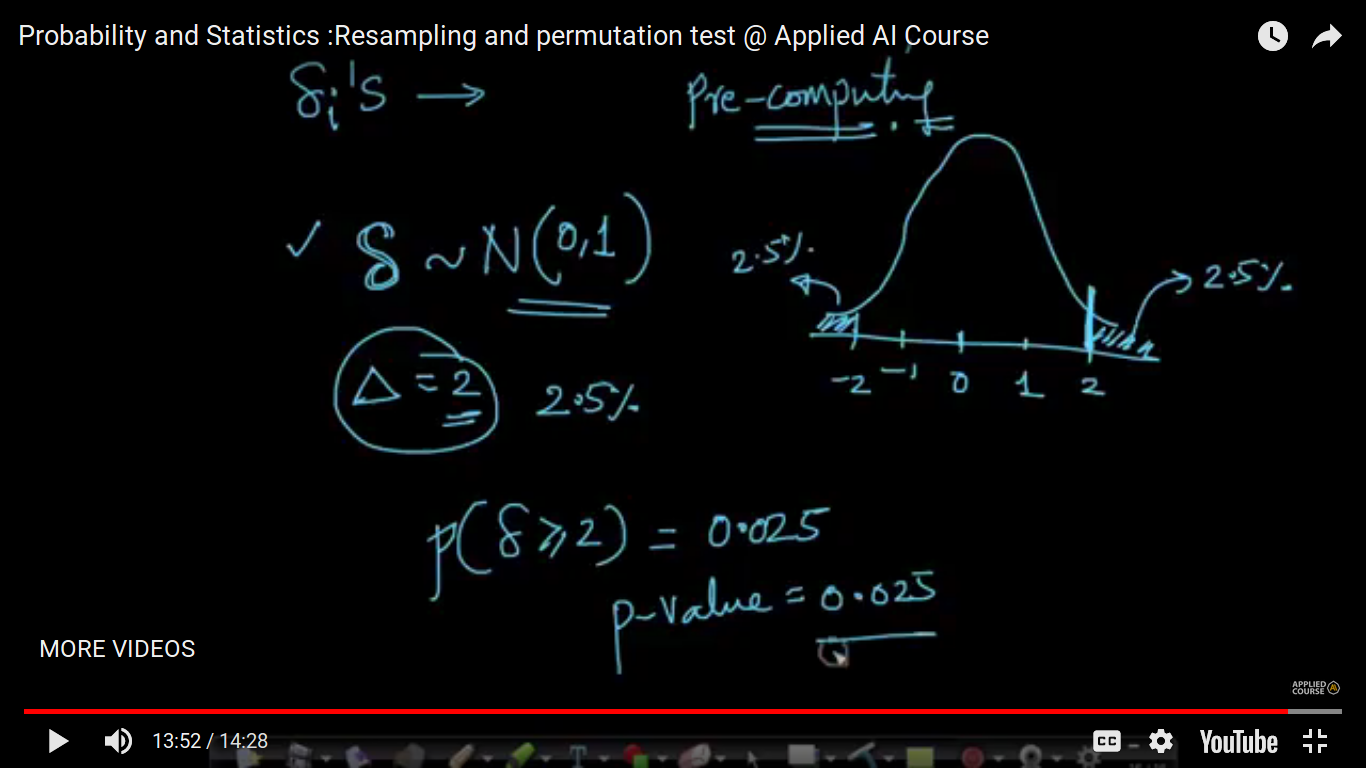
P-value is 20 percent i.e 0.2 means that there is 20 percent of my small delta(si) is greater than my large delta(triangle). where large delta(triangle) is the mu1-mu2 difference initially before shuffling. Here, we have 50+ 50 points. So, we have seen still there is a difference in small deltas. And hence it's not observed for large million values. To compute the p-value, we are assuming Ho i.e both classes doesn't have a difference an that's why we are jumble both the classes. And If the probability is very small(around 5%), we end with rejecting H0
Page 25
Want to create your own Notes for free with GoConqr? Learn more.