Descriptive Statistics

Descriptive Statitstics

Data Types

Quantitative

(Number of Dogs)

Allows Math Operation and slit in smaller values

Categorical

(Bred of Dogs)

Label a Gruop or Set of Ideas

Ordinal (Ordered)

Rating

Positive Neutral

Negative

Nominal

(No Order)

Breed

Poodel

Pug

Discrete

(Countable numbers)

0-1-2

Continuos

(Decimal Number)

Age of the dog in smaller values, like in years, months or days

0,1-0,2-1,5

The table below summarizes our data types. To expand on the information in the table, you can look through the text that follows.

Data Types

Quantitative:ContinuousDiscrete

Height, Age, IncomePages in a Book, Trees in Yard, Dogs at a Coffee Shop

Categorical:OrdinalNominal

Letter Grade, Survey RatingGender, Marital Status, Breakfast Items

Below is a little more detail of the information shared in the above table.

Another Look

To break down our data types, there are two main blocks:

Quantitative and Categorical

Quantitative can be further divided into Continuous or Discrete.

Categorical data can be divided into Ordinal or Nominal.

You should have now mastered what types of data in the world around us falls into each of these four buckets: Discrete, Continuous, Nominal, and Ordinal. In the next sections, we will work through the numeric summaries that relate specifically to quantitative variables.

Quantitative vs. Categorical

Some of these can be a bit tricky - notice even though zip codes are a number, they aren’t really a quantitative variable. If we add two zip codes together, we do not obtain any useful information from this new value. Therefore, this is a categorical variable.

Height, Age, the Number of Pages in a Book and Annual Income all take on values that we can add, subtract and perform other operations with to gain useful insight. Hence, these are quantitative.

Gender, Letter Grade, Breakfast Type, Marital Status, and Zip Code can be thought of as labels for a group of items or individuals. Hence, these are categorical.

Continuous vs. Discrete

To consider if we have continuous or discrete data, we should see if we can split our data into smaller and smaller units. Consider time - we could measure an event in years, months, days, hours, minutes, or seconds, and even at seconds we know there are smaller units we could measure time in. Therefore, we know this data type is continuous. Height, age, and income are all examples of continuous data. Alternatively, the number of pages in a book, dogs I count outside a coffee shop, or trees in a yard are discrete data. We would not want to split our dogs in half.

Ordinal vs. Nominal

In looking at categorical variables, we found Gender, Marital Status, Zip Code and your Breakfast items are nominal variables where there is no order ranking associated with this type of data. Whether you ate cereal, toast, eggs, or only coffee for breakfast; there is no rank ordering associated with your breakfast.

Alternatively, the Letter Grade or Survey Ratings have a rank ordering associated with it, as ordinal data. If you receive an A, this is higher than an A-. An A- is ranked higher than a B+, and so on… Ordinal variables frequently occur on rating scales from very poor to very good. In many cases we turn these ordinal variables into numbers, as we can more easily analyze them, but more on this later!

Analysis Mesure

Center

Shape

Outlier

Data points that fall very far from the rest of the values in our data set

Spread

(How far are point from anoather)

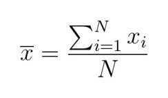
Mean

(Sum of all values divided by the count of values )

Mode

(Most frecuent number in the dataset)

Median

(The middle value of an ordered data set)

In a even data set u use de mean of de two numbers in de middle

Notation

Common math languaje used to comunicate

Random Varieable = X in Capitalcase

And observed Values in Lower Case Xsub1 = 5

Range

= Maximum- Minimum

Interquartile Range

(IQR)

= Q3-Q1

Standard Deviation

(Average difference of each observation from the mean of the data set)

Used to compere spread of difefrent groups

Varience

(Average squared difference of each observation from the mean)

Other Measures of Spread

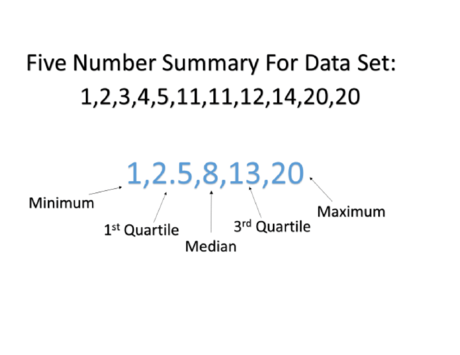
5 Number Summary

In the previous sections, we have seen how to calculate the values associated with the five number summary (min, Q_1Q1​, Q_2Q2​, Q_3Q3​, max), as well as the measures of spread associated with these values (range and IQR).

For datasets that are not symmetric, the five number summary and a corresponding box-plot are a great way to get started with understanding the spread of your data. Although I still prefer a histogram in most cases, box-plots can be easier to compare two or more groups. You will see this in the quizzes towards the end of this lesson.

Variance and Standard Deviation

Two additional measures of spread that are used all the time are the variance and standard deviation. At first glance, the variance and standard deviation can seem overwhelming. If you do not understand the equations below, don't panic! In this section, I just want to give you an overview of what the next sections will cover. We will walk through each of these parts thoroughly in the next few sections, but the big picture is to gain the following:

An understanding of how the mean and variance are calculated.

Intuition for why the calculations of the mean and variance make sense to capture the spread of our data.

Fields where you might see these values used.

Why we might use the standard deviation or variance as opposed to the values associated with the 5 number summary for a particular dataset.

Calculation

We calculate the variance in the following way:

\frac{1}{n}\sum\limits_{i=1}^n(x_i - \bar{x})^2n1​i=1∑n​(xi​−xˉ)2

The variance is the average squared difference of each observation from the mean.

In a spreadsheet application with 10 rows of data we would create a new column next to our data and type in =A1-AVG(A1:A10) and copy this down for all values. This would get us the difference between each data point and the Average of all the data. Then we type in the cell below this new column of differences from the Average =Sum(B1:B10)^2 here we are adding all these values together and then squaring them. We will cover using spreadsheets in the next section of this course.

The standard deviation is the square root of the variance. Therefore, the calculation of the standard deviation looks like the following:

\sqrt{\frac{1}{n}\sum\limits_{i=1}^n(x_i - \bar{x})^2}n1​i=1∑n​(xi​−xˉ)2​

The standard deviation is a measurement that has the same units as the rest of our data, and the units of the variance are the square of our original data.

In a spreadsheet application we simply add another cell beneath our variance measure and type in =sqrt(B11). We will cover using spreadsheets in the next section of this course.

Again, this section is aimed as a precurser to the information you will be covering on the next many sections. If it doesn't make sense on this first pass, do not worry. You will be working through this calculation, and building your intuition with Katie as you work through an example using the salary data. Then I will be back to provide some context about why these calculations are important, and where you might see them!

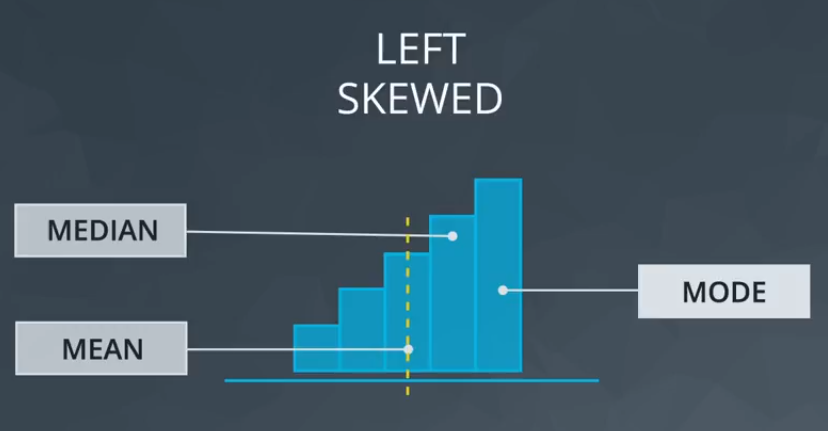
Left Skewed

Mean> Median

Mean pulled by the tail

Median closer to the Mode

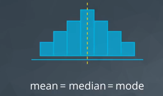
Normal Distribution

The Bell Curve

Mean==Median==Mode

Symemtric

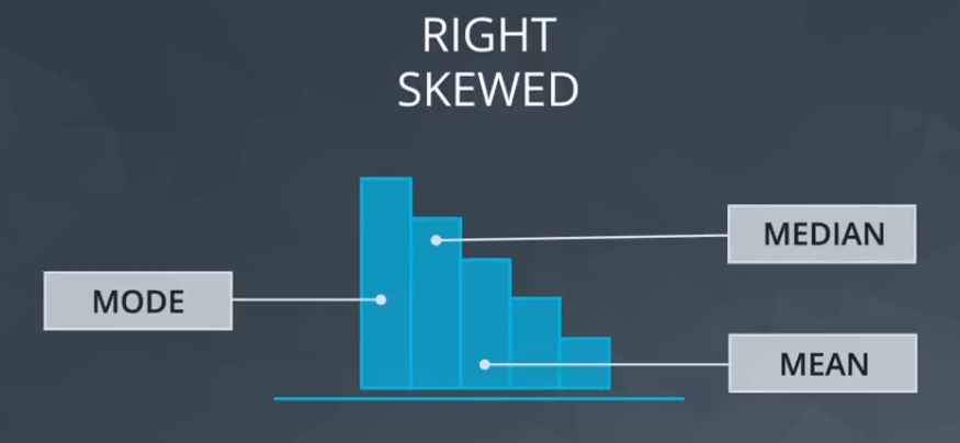
Right Skewed

Mean > Median

Mean pulled by the tail

Median closer to the Mode

1. Noting they exist and the impact on summary statistics.

2. If typo - remove or fix

3. Understanding why they exist, and the impact on questions we are trying to answer about our data.

4. Reporting the 5 number summary values is often a better indication than measures like the mean and standard deviation when we have outliers.

5. Be careful in reporting. Know how to ask the right questions.

Below are my guidelines for working with any column (random variable) in your dataset.

1. Plot your data to identify if you have outliers.

2. Handle outliers accordingly via the methods above.

3. If no outliers and your data follow a normal distribution - use the mean and standard deviation to describe your dataset, and report that the data are normally distributed.

Side note

If you aren't sure if your data are normally distributed, there are plots called normal quantile plots and statistical methods like the Kolmogorov-Smirnov test that are aimed to help you understand whether or not your data are normally distributed. Implementing this test is beyond the scope of this class, but can be used as a fun fact.

4. If you have skewed data or outliers, use the five number summary to summarize your data and report the outliers.