Probability

Probability

1. Axions

   • P(a) = 1
   • P(a) should be between 0 and 1
   • (In disjoin sets) P(a or b) = P(a) + P(b)
   • Prove [ P(AUB) =P(A)+P(B)-P(AB) ]
     • The union of two events, A U B, can be broken up into three sets:
       • A that are not in B (AB´)
       • B that are not in A (A´B)
       • Both A and B (AB)
       • Together, these three sets contain every element of AUB.
         • P(AUB) = P(AB´ U A´B U AB ).
         • The three sets on the right are disjoint, thereforeew it may aply the addition
           • P(AUB) = P(AB´) + P(A´ B) + P(AB).
           • Also P(A)
             • P(A) = P(AB´U AB) = P(AB´) + P(AB),
           • Also P(B)
             • P(B) = P(A´B U AB) = P(A´B) + P(AB),
           • A´B and AB are disjoint. Adding, we find
             • P(A) + P(B) = P(AB´+ P(A´B) +2×P(AB).
             • This would be P(AUB), but for the fact that P(AB) is counted twice, not once. It follows that, in general,
               • P(AUB) = P(A) + P(B) - P(AB).

2. Experiment

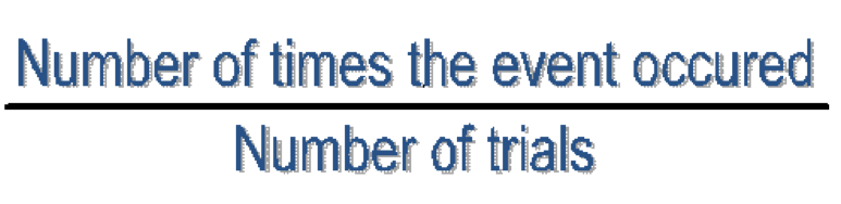
   • The ratio of the times an event occurs over the trials

3. Sample space

   • The sample space of an experiment is the set of all possible outcomes of that experiment.
   • Example
     • What is the probability of each outcome when a dime is tossed?
       • The outcomes of this experiment are head and tail.
         • Probabilities:
           • P(tail) = 1/2
           • P(head) = 1/2
         • Sample space:
           • Head
           • Tail

4. Event

   • Set of outcomes of an experiment
   • Example
     • A deck of 52 playing cards
       • Red/ black at the same without being a joker
         • Probability= 0
         • Event= {}
       • The 5 of Hearts
         • Probability = 1
         • Event = {5-hearts}
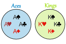
       • A King
         • Probability = 4
         • Event= {K♥, K♠, K ♦, K♣ }
   • Mutually exclusive
     • Cant happen at the same time
     • Are dependent
       • Because one situation may happen without the other
   • independent events
     • Two events, A and B, are independent if the fact that A occurs does not affect the probability of B occurring.
     • Multiplication rule
       • P(A and B) = P(A) · P(B)
   • Conditional probability
     • When two events, A and B, are dependent, the probability of both occurring is
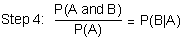
     • The Conditional Probability of an event can be derived from Multiplication Rule:
       • Multiplication rule
       • Divide both sides
       • Cancel P(a)
       • Commute the equation
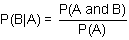
       • Formula
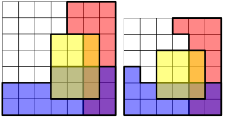
     • These are two examples illustrating conditional independence
       • Each cell represents a possible outcome.
         • The events R, B and Y are represented by the areas shaded red, blue and yellow respectively. The overlap between the events R and B is shaded purple.
           • R and B are conditionally independent given Y because:
             • but not conditionally independent given not Y because: :
   • Complementary event
     • P(A´ ) = 1 − P(A).
       • Proof
         • They are
           • A ∪ A´ = S
           • A ∩ A´ = ∅
           • Therefore, by Axiom theory
             • P(A ∪ A´ ) = P(A) + P(A´ ) = 1
             • Since P(A ∪ A´) = P(S) = 1, whence P(A´) = 1 − P(A).
   • Can´t extend to 1
     • Because the maximum will be the s/s which will be 1 and if it increases it would have a decimal which is imposible

5. Law of total

   • Is a fundamental rule relating marginal probabilities to conditional probabilities

6. Bayes theorem

   • Describes the probability of an event, based on prior knowledge of conditions that might be related to the event.
   • Example
     • Cancer of 65
       • Cancer = General prevalence of cancer
         • 1%
       • Writing C for the event "having cancer"
         • P(C)=0.01
       • Suppose also that the probability of being 65 years old is 0.2%
         • P(65)=0.002
         • Knowing this, we can calculate the probability of having cancer as a 65-year-old by applying Bayes' formula:

7. Example

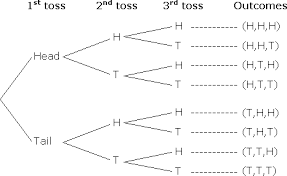
   • Sample space when 1,2 and 3 coins are thrown
     • {HHH, HHT, HTH, HTT, THH, THT, TTH, TTT}
   • Sample space when 2; 6 sided dice
     • {1-1, 1-2, 1-3, 1-4, 1-5, 1-6, 2-1, 2-2, 2-3, 2-4, 2-5, 2-6, 3-1, 3-2, 3-3, 3-4, 3-5, 3-6, 4-1, 4-2, 4-3, 4-4, 4-5, 4-6, 5-1, 5-2, 5-3, 5-4, 5-5, 5-6, 6-1, 6-2, 6-3, 6-4, 6-5, 6-6}

8. Fundamental counting principle

   • When there are m ways to do one thing, and n ways to do another, then there are m×n ways of doing both.
   • Example
     • You have 3 shirts and 4 pants.
     • That means 3×4=12 different outfits.

9. Throwing dice

   • When throwing the amount of dices needed its the same as telling to throw one time the amount of dices, it will have the same probability.

10. Probability distribution

    • A function of a discrete variable whose integral over any interval is the probability that the variate specified by it will lie within that interval.

11. Random variable

    • Usually written X, is a variable whose possible values are numerical outcomes of a random phenomenon. There are two types of random variables, discrete and continuous.

12. Binomial diastribution

    • The binomial distribution function specifies the number of times (x) that an event occurs in independent trials .
    • Conditions
      • The number of observations n is fixed.
      • Each observation is independent.
      • Each observation represents one of two outcomes ("success" or "failure")
      • The probability of "success" p is the same for each outcome.
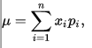
    • Mean
      • is a binomially distributed random variable, n being the total number of experiments and p the probability of each experiment yielding a successful result, then the expected value of X is:[3]
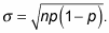
    • Standart deriviatiuon

13. Normal distribution

    • A normal distribution in a variate with mean and variance is a statistic distribution with probability density function.
    • Areas under normal distribution
      • Areas under portions of a normal distribution can be computed by using calculus. Since this is a non-mathematical treatment of statistics, we will rely on computer programs and tables to determine these areas.

14. Z- score

    • z = (x – μ) / σ

15. Standard normal distribution

    • As discussed in the introductory section, normal distributions do not necessarily have the same means and standard deviations.
      • mu = 0 and sigma =1
      • mu and sigma are other than 0 and 1
        • Sigma level

Images and files in the map