Fichas

AP Statistics Exam Review

Emily Lu Math 7th grade Inglés 191 fichas

Fichas del conjunto (191)

1Categorical Dataqualitative data that identifies characteristics (hair color, preferences, etc).
2Numerical Dataquantitative data; split into discrete (counts) and continuous (measurements).
3Uni-variate Datadata that describes 1 characteristic of a population.
4Bi-variate Datadata that describes 2 characteristics of a population.
5Multivariate Datadata that describes >2 characteristics of a population.
6Relative Frequency Formulafrequency/n * 100
7Interquartile Range (IQR)Q3 - Q1
8Describing Categorical DataIdentify the highest frequency and lowest frequency,
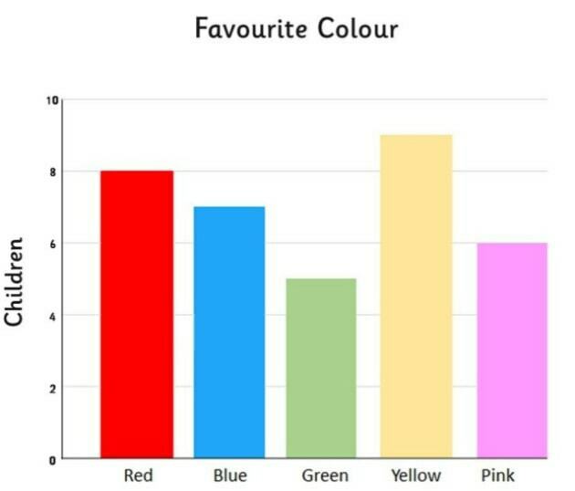
9Name this graph and identify the type of data it's used forBar Chart, Categorical Data
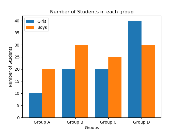
10Name this graph and identify the type of data it's used forDouble Bar Chart, Categorical Data w/ 2 or more Groups
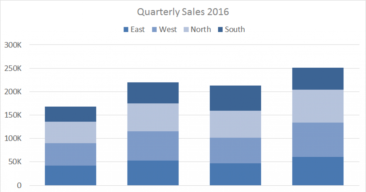
11Name this graph and identify the type of data it's used forStacked Bar Chart, Categorical Data (% to whole relationship)
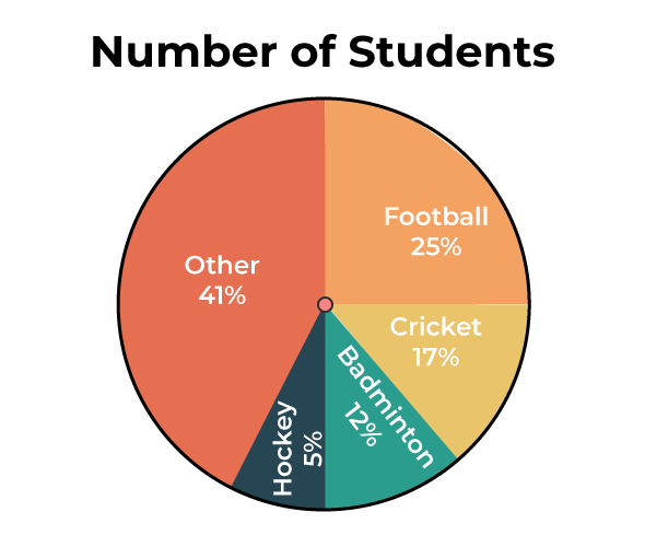
12Name this graph and identify the type of data it's used forPie Chart, Categorical Data (relation of part to whole)
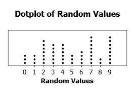
13Name this graph and identify the type of data it's used forDot Plot, Discrete Numerical Data
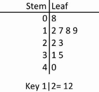
14Name this graph and identify the type of data it's used forStem-and-Leaf Plot, Univariate Numerical Data
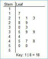
15Name this graph and identify the type of data it's used forSplit Stem-and Leaf Plot, Univariate Numerical Data w/ long list of leaves
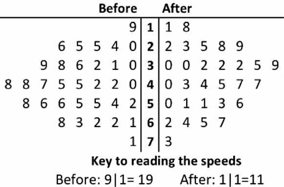
16Name this graph and identify the type of data it's used forBack-to-Back Stem-and-Leaf Plot, Univariate Numerical Data w/ 2 Grou[s
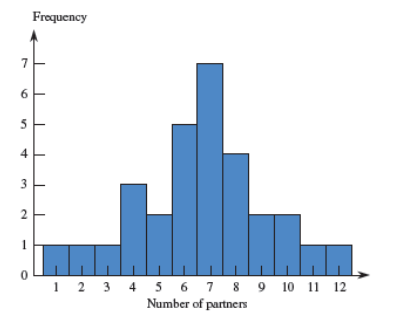
17Name this graph and identify the type of data it's used forDiscrete Histogram, Univariate Discrete Numerical Data
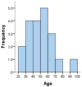
18Name this graph and identify the type of data it's used forContinuous Histogram, Univariate Continuous Numerical Data
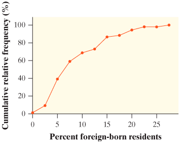
19Name this graph and identify what it's used forCumulative Relative Frequency Plot, Percentiles
20Parameterfixed value about a population.
21Statisticcalculated value from a sample.
22Degrees of Freedom# of observations free to vary; n - 1
23Left-Skewedtail on the left.
24Right-Skewedtail on the right.
25Uni-modal1 peak.
26Bi-modal2 peaks.
27Multimodal>2 peaks.
28Linear Transformation Rule+/- constant changes the mean.
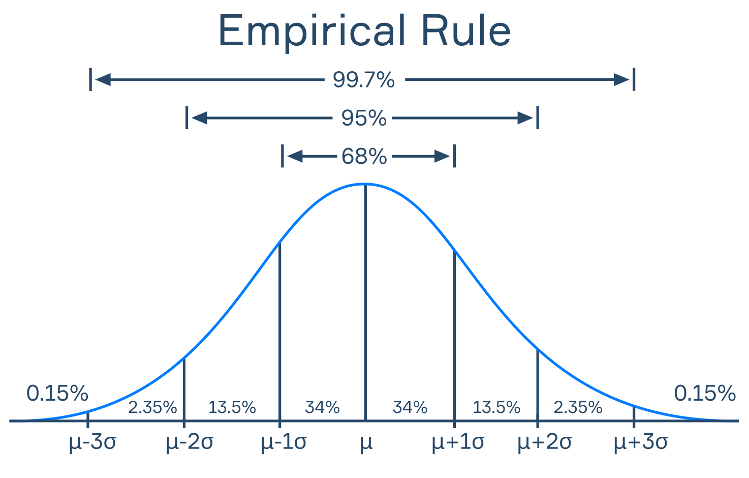
×/÷ a constant changes BOTH the mean and SD.
29Empirical Rule68% of values are within 1 SD of the mean.
95% of values are within 2 SD of the mean.
99.7% of values are within 3 SD of the mean.
30Combining Meansµa+b = µa + µb
µa-b = µa - µb
31Combining Standard Deviationsσa±b = √σ²a + σ²b
32Trimmed Mean1. List values in order.
2. Do % trimmed(n)
3. Remove that many observations from BOTH ends.
4. Calculate mean with the new data set.
33Boxplot Outliersany values < Q1 - 1.5(IQR) or > Q3 + 1.5(IQR)
345 Number Summary1. Minimum
2. Q1
3. Median
4. Q3
5. Maximum
35Describing Numerical Data(SUCS)
Shape
Unusual values
Center
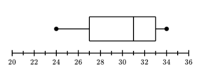
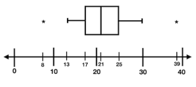
Spread
36Name this graph and identify the type of data it's used forBoxplot, Univariate Numerical Data
37Name this graph and identify the type of data it's used forModified Boxplot, Univariate Numerical Data
38Identify the concept that this image displaysEmpirical Rule
39Countinghow many ways can an event occur? (order matters/doesn’t)
40Permutationorder ALWAYS matters.
41Combinationrder DOESN'T matter.
42Union (A ∪ B)the event of A OR B happening
43Intersection (A ∩ B)the event of A AND B happening
44Disjoint (Mutually Exclusive)2 events have no outcomes in common.
45Independentone event occurs and doesn’t change the probability of another event
46Hypothetical 1000suggests that the overall total will be 1000; used for probability tables only.
47Permutation Formulamath → prob → nPr
48Combination Formulamath → prob → nCr
49Disjoint Union FormulaP(A ∪ B) = P(A) + P(B)
50Non-Disjoint Union FormulaP(A ∪ B) = P(A) + P(B) - P(A ∩ B)
51Independent Intersection FormulaP(A ∩ B) = P(A) x P(B)
52Not-Independent Intersection FormulaP(A ∩ B) = P(A) x P(B|A)
53Probability Formula (Equallly Likely Outcomes)favorable outcomes/total outcomes
54Conditional ProbabilityP(B|A) = P(A ∩ B)/P(A)
55At Least One FormulaP(at least one) = 1 - P(Aᶜ)
56Exactly One FormulaP(exactly one) = P(A ∩ Bᶜ) + P(Aᶜ ∩ B)
57Explanatory Variablex-value/independent variable/causes the change.
58Response Variabley-value/dependent variable/the outcome of the change.
59Correlationrelationship between bivariate variables, whether positive/negative
60Correlation Coefficient (r)a quantitative assessment of STRENGTH and DIRECTION of a LINEAR relationship.
61Least Squares Regression Line (LSRL)the line of best fit, defined by ŷ = a + bx
62Extrapolationthe LSRL can’t be used for predictions made outside the range (too high/too low).
63Coefficient of Determination (r²)the proportion of variation in y determined by the linear relationship between x and y
64Residualvertical deviation between a point and the LSRL; y - ŷ
65Residual Plota scatter plot of (x, residual) pairs, determining whether a linear model is appropiate (linear pattern) or not (not a linear pattern).
66Influential Pointa point that if removed, changes the slope, y-intercept, and/or correlation substantially
67High Leverage Pointan influential point that changes the slope/y-intercept, affecting the LSRl directly.
68Outlieran influential point that changes r.
69a (y-int) Formulaa = ȳ - bx̄
70b (slope) Formulab = r(Sy/Sx)
71Interpreting the Correlation Coefficient (r)"There is a (weak/moderate/strong) (negative/positive) linear relationship between x and y."
72Interpreting the Slope"For a one unit increase in x, there is a predicted (increase/decrease) of b in y."
73Interpreting the Coefficient of Determination (r²)"Approximately r²% of the variation in y is explained by the LSRL of x on y."
74Identify the type of plot based on this imageScatter Plot
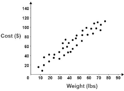
75Censusa complete count of the population.
76Sampling Designmethod used to choose a sample from the population.
775 Types of Sampling Design1. Simple Random Sample (SRS)
2. Stratified Random Sample
3. Systematic Random Sample
4. Cluster Sample
5. Multistage Sample
78Sampling Framea list of every individual in the population.
79Simple Random Sampleeach individual/set of individuals has an EQUAL chance of being selected
80Stratified Random Samplepopulation is divided into STATA. An SRS is taken from each strata.
81Systematic Random Samplerandomly selects a BEGINNING POINT and follows a systematic approach.
82Cluster Samplerandomly picks a location and samples ALL from there.
83Multistage Samplesplits the process into stages and takes an SRS at each stage.
84Biasa systematic error in measuring the estimate; often favors certain outcomes.
856 Types of Bias1. Voluntary Response
2. Convenience Sampling
3. Undercoverage
4. Nonresponse
5. Response Bias
6. Wording of Questions
86Voluntary ResponseSELF-SELECTION; people choose to respond because they have strong opinions.
87Convenience Samplingasking the easiest people to participate.
88Undercoveragewhen certain groups from the population are left out of the selection process.
89Nonresponsewhen an individual chosen refuses to participate/can’t be contacted.
90Response Biaswhen the respondent/interviewer causes bias by giving the wrong answer.
91Wording of Questionsthe use of big words/connotation can cause bias through confusion and indirect persuasion.
92Observational Studyobserving outcomes WITHOUT treatment.
93Experimentobserving outcomes AFTER treatment.
94Surveysimply asking respondents for data; NO observations or treatment.
95Experimental Unitthe individual to which the different treatments are assigned.
96Factorx; what are we testing?
97Response Variabley; what are we measuring?
98Levela specific value for the factor that splits it into different categories.
99Treatmenta specific experimental condition applied to the units.
100Control Groupa group used to compare the factor against.
101Placebodummy treatment with no effect.
102Blindingexperimental units don’t know which treatment they’re getting.
103Double Blindneither the experimental units nor the evaluator know which treatment was used.
104Confounding Variableoutside variable that affects the outcome but wasn’t considered in the beginning.
105Blockhomogeneous group formed by experimental units that share similar characteristics.
1063 Types of Experimental Design1. Completely Randomized
2. Randomized Block
3. Matched Pairs
107Completely Randomizedexperimental units are assigned randomly to treatments.
108Randomized Blockexperimental units are blocked into homogeneous groups. Then, they are randomly assigned to treatments.
109Matched Pairsunits are paired up; one gets treatment A and the other automatically gets treatment B. OR, every experimental unit gets both treatments in a random order.
1105 Parts of a Simulation1. Model
2. Trial
3. Assumptions
4. Chart
5. Conclusion
111ModelRandom Digit Table
“Let (digits) represent _______. “
112Trial“I will select (# of single digit/double digit numbers) to represent (each unit/group). I will record ____ and perform 5 trials.”
113Assumptions"P(probability) = #"
List all probabilities.
114ChartDraw a chart displaying the trials and what you're testing. Then, sum up your results and divide it by the number of trials to achieve your approximately results.
115Conclusion“Based on my simulation, I estimate… (approximate results).”
116Binomial Distributiontests for the number of successes that can occur out of a given number of trials.
117Geometric Distributiontests for the number of trials until the 1st success is reached.
118pdfused when looking for exact values; P(X = x)
119cdfused when looking for cumulative values; P(X /≥ x)
120Mean of Linear Functionμᵧ = a + b(μₓ)
121Standard Deviation of Linear Functionσᵧ = |b|σₓ
122Unusual Distributiona continuous distribution with uniquely shaped density curve composed of triangles, rectangles, and/or trapezoids.
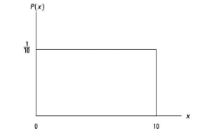
123Uniform Distributionan evenly distributed continuous distribution; shaped as a rectangle.
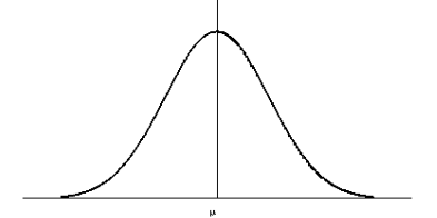
124Normal Distributiona continuous distribution with a symmetrical bell-shaped density curve defined by the mean and standard deviation.
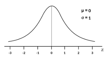
125Standard Normal Distributiona normal distribution with mean of 0 and standard deviation of 1.
126Normal Probability Plota scatter plot used to assess normality; linear pattern = distribution is approximately normal.
127Trapezoid FormulaA = 1/2(b1+b2)h
128Rectangle FormulaA = bh
129Triangle FormulaA = 1/2bh
130Height of Uniform Dist.1/(b - a)
131Probability of Uniform DistributionA = bh
132Mean of Uniform Dist.μₓ = (a+b)/2
133Standard Deviation of Uniform Dist.σₓ = √((b-a)²/12)
134Probability of Normal Dist.normcdf(l, u, μ, σ)
135X-value of Normal Dist.invNorm(a, μ, σ)
136Standardization Formulaz = (x -μ)/σ
137When SD increases, what happens to the normal curve?It flattens and spreads out.
138When SD decreases, what happens to the normal curve?It becomes narrower and thinner.
139Identify the type of density curve based on this imageUnusual Density Curve
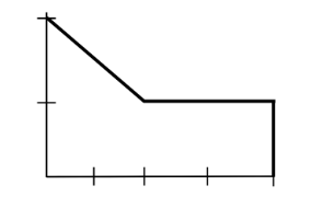
140Identify the type of density curve based on this imageUniform Density Curve
141Identify the type of density curve based on this imageNormal Density Curve
142Identify the type of density curve based on this imageStandard Normal Density Curve
143Sampling Variabilitythe observed value of the statistic depends on the particular sample selected from the population.
144Point Estimatestatistic used to estimate a parameter; often not close to the true value of the parameter.
145Confidence Intervalinterval of possible values for the population characteristic.
146Confidence Levelthe success rate of all confidence intervals that contain the true proportion p.
147Confidence Interval Default Formulapoint estimate ± critical value(standard error)
148Z-score Formula1. (1 - CL)/2 = a
2. 2nd → vars → invNorm(a, 0, 1, left) → Use the POSITIVE vers.
149p̂number of successes/n
150Null Hypothesis (H0)a claim about the parameter initially assumed to be true.
151Alternate Hypothesis (Ha)competing claim against the null; what you are trying to prove.
152Test Statisticindicates how many standard deviations the statistic is from the parameter.
153P-valuethe probability of obtaining a test statistic as inconsistent as the null hypothesis, assuming it’s true.
154Level of Significance (α)he probability that we REJECT the null hypothesis, assuming it’s true.
155Test Statistic Default Formula(statistic - parameter)/standard error
156P-value for Proportions2nd → vars → normcdf(l, u, 0, 1)
157np TestsIf np ≥ 10 and n(1-p) ≥ 10), the sampling distribution is approximately normal.
158Type I Errorrejecting the null hypothesis when it’s true; denoted by alpha (α).
159Type II Errorfailing to reject the null hypothesis when it’s false; denoted by beta (β).
160Consequencesthe outcomes of making Type I/Type II errors.
161Relationship between α and βα and β are inversely related; as α gets bigger, β gets smaller, vise versa.
162Powerthe probability that the test rejects the null hypothesis when the alternate hypothesis is true (CORRECT).
163What happens if alpha increases?Power increases, Type I Error increases, and Type II decreases.
164What happens if n increases?Power increases and Type II Error decreases.
165What happens if P0 - Pa increases?Power increases and Type II Error decreases.
166np Tests (2-Prop)If n₁p₁ ≥ 10, n₁(1-p₁) ≥ 10), n₂p₂ ≥ 10, and n₂(1 - p₂) ≥ 10, the sampling distribution is approximately normal.
167Central Limit Theoremwhen n ≥ 30, the sampling distribution can be approximated by a normal curve.
168t Distributiona continuous distribution based on df; used when σ s unknown.
169df (t-Dist)df = n - 1
170P-value for Means2nd → vars → tcdf(l, u, df)
171T-score Formula1. (1 - CL)/2 = a
2. 2nd → vars → invT(a, df) → Use the POSITIVE vers.
172Central Limit Theorem (2-Samp)when n₁ ≥ 30 and n₂ ≥ 30, the sampling distribution can be approximated by a normal curve.
173Pooled t Inferenceused when the variances of 2 populations are equal; σ₁ = σ₂
174df (Matched Pairs)df = n - 1
175df (2-Samp)Use 2-SampTTest and truncate the value.
176kthe number of categories.
177χ² testtests the counts of CATEGORICAL data; the 3 types are GOF, homogeneity, and independence
178GOF testmeasures univariate data for a single sample; uses a ONE-WAY table.
179Homogeneitymeasures univariate data for TWO/MORE SAMPLES; uses a two-way/more table.
180Independencemeasures BIVARIATE data for two/more samples; uses a two-way/more table.
181Expected Counts (GOF)n(proportion)
182Expected Counts (Homoegeneity and Independence)Make a matrix and use χ²-Test
183df (GOF)df = k - 1
184df (Homogeneity and Independence)df = (r- 1)(c - 1)
185P-value (Chi-squared)2nd → vars → χ²cdf(χ2, ∞, df)
186Identify the type of distribution based on this imageχ² Distribution
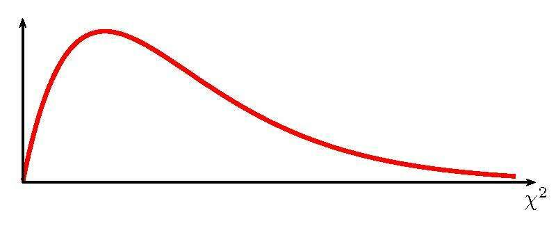
187Deterministic Relationshipa relationship in which the value of y is determined by the value of x.
188Error Variable (e)a random deviation that causes observed (x, y) points to avoid falling exactly on the population regression line.
189Test Statistic (LinReg)t = b/sb
190P-Value (LinReg)2nd → Vars → tcdf(l, u, df)
191df (LinReg)df = n - 2