Advanced Statistics

Page 1

Research Design and Statistics

Each IV can be one of two types of design:

Repeated measures / within subjects

Independent measures/ between subjects

Page 2

Page 3

Type I and type II errors

Type I error

Finding a significant result when in fact there is no difference

Type II error

Finding a non-significant result when in fact there is a difference

We cannot know if we have made one of these errors

But smaller p-values mean Type I error is less likely

Page 4

Parametric tests: Assumptions

Normal distribution of residuals

Eyeballing histograms or residual plots,

Statistical tests

If violated use a non-parametric test (if there is one)

Homogeneity of Variance

Each independent group should have similar spread of data (variance)

Check using Levene’s test

f violated use a non-parametric test or transform your data

Sphericity (special case of homogeneity of variance for repeated measure with more than 2 levels)

Check using Mauchly’s test

If violated use corrected values (and to be safe you can just always do this)

Page 5

T-tests

Look for a difference between means

Use with ONE IV with TWO levels/conditions

Two main types of t-test

Independent samples t-test:

used when your IV is INDEPENDENT samples

2. Paired samples t-test:

used when your IV is REPEATED samples

With both types of t-test: t(df) = t value, p = sig. value, d = ?

Page 6

ANOVA

We have ONE IV with MORE than TWO levels/conditions

One-way ANOVA: One IV with 3+ conditions

OR

We have MORE than ONE IV

Two-way ANOVA - Two IV’s with 2+ conditions

Three-way ANOVA - Three IV’s with 2+ conditions

N-way ANOVA…

Design:

Independent / between subjects ANOVA

– all IV’s are independent measures

Repeated / within subjects ANOVA

– all IV’s are repeated measures

Mixed measures ANOVA

– some IV’s are independent measures, some are repeated measures

Report F(df for the effect, df error)=F value, p=sig. value, etasquared.

Page 7

Variance

UNSYSTEMATIC VARIANCE

Looking at the deviation of each point to the group mean (residual) – gives us variance for each group

SYSTEMATIC VARIANCE

Differences between each mean and the grand mean tells us how far away each mean is from being the same

ANOVA

Hence ANOVA uses the:

Differences between each group mean and the grand mean to work out systematic variance

Differences between each individual data point and the group mean of that point to work out unsystematic variance

F (F-ratio test) which is the test statistic used by ANOVA is: F = systematic variance unsystematic variance

Page 8

ANOVA:

Main effects and interactions

Main effects

Tells you whether there is a difference between the conditions of your independent variable

When there are 2+ IV’s, main effects are reported for each IV

Interactions

Only given when there are 2+ IV’s

Looks at the whether the effect of one IV depends on the level of another.

Another way of thinking about interactions: differences between sub-groups are different in different groups.

Page 9

ANOVA: Post-hoc tests

A significant finding tell us that there is a difference, but where is the difference?

Compares each level with each other level

Like running multiple t-tests

But post-hocs are corrected for elevated chance of a Type I error

Bonferroni correction

p value multiplied by the number of comparisons

Page 10

Effect size

Total amount of variance in the DV that is explained by the IV

How is this different from p?

The p value relates to the strength of evidence for the existence of an effect, not how big the effect is

The effect size looks at how much of the variance is explained on a standardised measure by the manipulation

Page 11

Confidence interval on the effect size

If the confidence interval on the effect size excludes zero, then we are confident there is an effect.

Here, we are only confident Intervention 1 is effective

Page 12

Regression

Regression lets us ask and answer ‘what is the best predictor of…’ or ‘by how much will the outcome change if predictor changes?’

outcome = (coefficient * predictor )+ intercept

The predictor variable is plotted on the x axis

The outcome variable is plotted on the y axis

The coefficient of “the predictor” is the slope of the line

The intercept is the value at which the line crosses the y axis

Useful properties of a General Linear model, given enough data, the numbers of both categorical and continuous predictors are theoretically unrestricted.

Page 13

Simple regression

To keep it simple, we’ll start out with just one predictor: advertising budget.

This essentially says how well the predictor predicts the DV

It is the proportion of variability in the DV that is explained by the predictor

What percentage of the variation in Ticket Sales can be predicted from knowing the Advertising Budget?

Adjusted R square value: 31% of the variation in Ticket Sales is predictable from knowing Advertising Budget

Looking at your results

ANOVA table tells us

Does the predictor have predictive power over the outcome?

Does the advertising budget predict the ticket sales?

should this be significant ( p < .05) it says the regression equation does explain a significant amount of the variation

Page 14

Multiple regression:

Each of the Sig values tell us whether that predictor is contributing significantly to the model

Standardised coefficients Beta tells us which predictor contributes most to the outcome

When running a multiple regression analysis which of the following assumptions are important? Multi-collinearity, dependent variable at interval

Page 15

Linearity

Linear regression. General linear model.

This means a straight line.

Most easily checked visually by plotting residuals

Page 16

For checking homogeneity of variance and normality

Many different types of histograms and scatter plots that can be looked at.

For you just two are important:

– Histogram of residuals for checking normal distribution

– Scatter plot of residuals against fitted/predicted values, for checking homogeneity of variance (other problems can also be detected)

Page 17

Confidence Intervals

Give an indication of the true likely effect of a population

95% confidence intervals

Give us a range (direction of effect)

Neg (harmful), Trivial, Positive (beneficial)

Populationally mean is between this range

Page 18

Nominal

Distinct categories are represented

No relationship or order between them

Called binary when just 2 categories

Ordinal

Ordered categories or ranked items

However, size of difference is not meaningful

Interval

Data you can measure

The size of difference between values is meaningful

Ratio

Meaningful definition of zero value

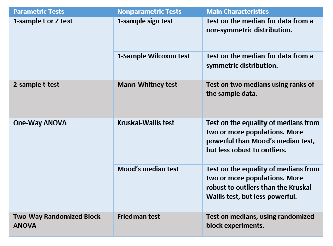
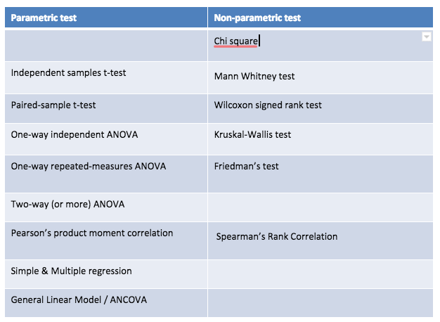
Nominal and ordinal are non-parametric statistics (do not use a T-test).

Ratio and interval a parametric test is possible.

Page 19

Page 20

Best Test Flow Chart (application/pdf)