
Mind map
Data analysis Practical part
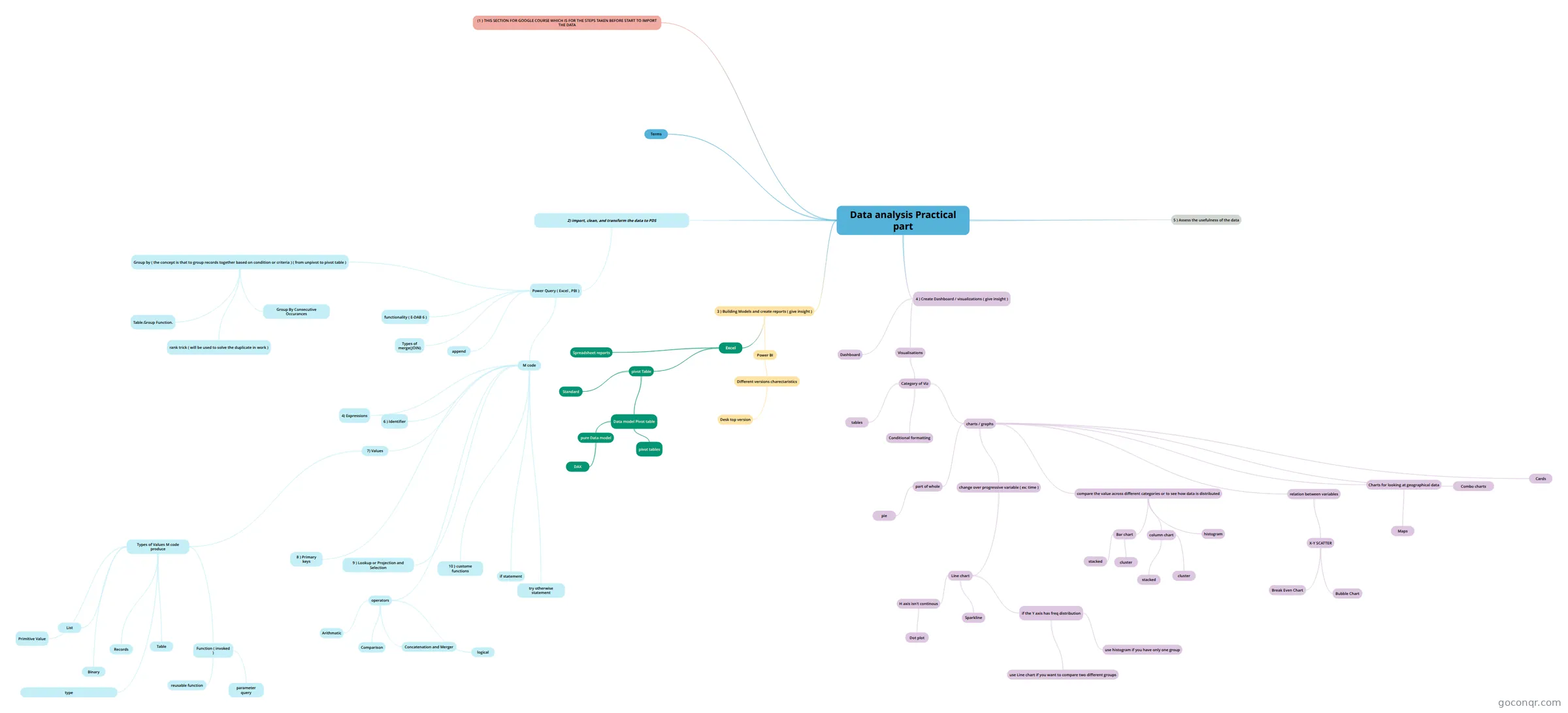
Mind map: Data analysis Practical part
Map content
Data analysis Practical part
- Transfer the row data into useful and refreshable information for the decision makers to take BI decision because it was built on BI
- • Name all tables, fields, queries and other items with smart and consistent names.
2) import, clean, and transform the data to PDS
- PDS is the base of every thing that will be built on it, like reports / dashboards / viz
- condition for the ideal PDS : - each data in separate column to let the data analytics tools work - 1st row is the columns' header define the data goes into the column - each subsequent row contain one data point - check if the data analytics tool you are using need the PDS data type to be explicitly declared and amend the data type to correct form. - name the tables always smarlty.
- - in case we use Excel for PDS, transform the PDS to excel table because Power tools require that, and it gives the dynamic feature to it.
- Power Query ( Excel , PBI )
- functionality ( E-DAB 6 )
- 3 - load the PDS to A ) Excel Sheet . B) PivotTable Cache C) Power Pivot Data Model
- 4- PQ require the data to be in excel table format before importing it Data --> from table/range --> from table
- to look up at the queries that already made , we will open the Query Pane ( like PIVOT TABLE window ) Data ---> queries and connections
- we can clean the data in excel in 3 main ways , but the PQ is the best - formulas ( like what i do ) - flash fill ( in case we need to clean the data only one time ) - PQ
- why PQ is the best : 1- easier when the cleaning is complicated or has multiple steps 2-easier when the data are from external source 3- can combine multiple files to one PDS 4- the PQ is linked to the final report/viz , when we amend anything in it , just refresh and it will reflect
- - we must designate the correct data type in PQ ” to indicates what sort of data can go in a particular Field or Column.
- data types could be - Text : only text value - data : onyl date value- Whole Number - no decimels - currency : currency amount with up to 4 decimls
- If you do not choose the correct data type for each column, the data analysis features like PT or PBI will not work properly ex: A Sales Column without a number Data Type may not be able to be summed.
- To change the Load locations (like change from PivotTable Cache to Excel Table in Worksheet) PQ pane ----> right click -----> load to
- Action Notes : to import a data table from Excel workbook to PQ transfer the data table to Excel table format ----> data ---> from table/range in case the data putted in one column , after you go to PQ editor Home ----> split column ----> by delimiter ( for this case ) ---> check the data type and remane the columns header
- Action Notes : to import a data table from Text/csv file to PQ Data ---- > get data --- > from file ----> from text/csv ----> search for desired file ----- check the preiveiw and confirm the delimiter ----> Transform
- General Notes in PQ editor - always Name the query first thing , also remove the change data type step - use the first Row as columns header if needed - check the data type - you can amend the data source file if you need ( like file path )
- to know what is the delimiter from the text/csv file right click on the txt/csv file ----> open with Word
- Action Notes : to import and append data into one PDS ( if the file is 1 object only ) Data --> get data ----> from folder -----> navigate the folder ----> edit ----> amedn the extention text ( filter and choose the lower case for example ) ----- > highlight the first column then remove the remaining columns ---> combine and load to
- - when we need to mention a folder with excel sheets in it as data source, first we need to click on ( Transform ) not ( Load ) , then PQ Editor lists the files in the Content column and attributes about the files in subsequent columns. because excel is not like txt or csv file which has one object in it , Excel files can have many objects in one file (like Sheet objects, Table objects, Defined Names objects and so on) we cannot click the combine button (like we did in E-Dab Video #6 when we combined/appended Text Files). Instead, as intermediate step we have to add a Custom Column and use the Excel.Workbook function ( M code ) to extract the objects in the Excel File. The Custom Column button is in the Add Column Ribbon Tab in the Power Query Editor,
- after adding custom column remove the content column -> expand -> select data -> uncheck ( use the original column .......) --> check the preview at the buttom to make sure of the data . then , click expand again ---> ok then , add a correct data type to each column
- Name the Query you always do with different name than the source excel tables name
- What is great about using Power Query to import data from a Relational Database, like the Access Relational Database like in the above picture, is that when you import the tables, Power Query will import that tables and the Relationships. The fact that the Relationships are also imported is that we can then use the Relationships to help make our Transformations in Power Query easier to complete.
- snow flakes schema ( 2 d tables can be merged into one d) ===> Star schema when we need to go from snow flakes schema to Star schema , we need to merge the 2 d tables that cause the snow flakes schema , so we go to Many side ( of the 2 d tables ) and expand the matching column from the ONE side so now we have 1 perfect d table and we can delete the ONE side table to use star schema ( d tables connected to main f table )
- it is prefered to clear relations between PDS before load the data to PP or PBI and then link the tables in PP or PBI . example , when we got the PDS that have had relations in Access to PQ , we merged the PDS we want ( 2 d tables ) and merged (1 d with 1 f to add the product name in f table) then we load the data to PP or PBI then we linked back the tables by relationship , this more orgnized .
- Convert to lowercase. Because Power Query is Case Sensitive, and because we might get Text Files with extensions that have lowercase or uppercase letters, we need to convert all the Extensions to lowercase. We can do this by right-clicking the Extension Column, Point to Transform, then click on lowercase
- this is an example can be applied to all extentions types In order to only import the correct Text Files, we need to filter the Extension Column to only include files that contain “.txt”. To do this, click the dropdown arrow in the Extension Column, then point to Text Filters and then click on Equals.
- files with many objects (sheets , tables, print area..etc.) in it is being extracted by custom column and M code ( ex : EXCEL ) then appended steps : import from folder ==> manage the extention issues ( lowercase, filter ) ==> clean the file name (to know what data related to which ) then rename it ==> we need to remove all columns except the Content and cleaned columns ===> extract the objects with M code ===> remove the Binary column ==> expand the extracted column == > Name & item column refer to the object name , Kind column refer to the object kind , Data column contains the object's data == > filter what kind of object do you want ==> do EXACT filter in Name column if necessary to narrow the type of sheets desrired for example ===================================== files that have only 1 object like Text/csv files we can append directly
- If we Load the Power Query Transformation to an Excel Sheet, we have to perform two separate Refreshes: 1. First Refresh the Query. 2. Second Refresh the PivotTable
- If we Load the Power Query Transformation to a PivotTable (option in the Import Data dialog box), all we have to do is refresh the PivotTable one time,
- UNPIVOT crosstable report to PDS ( only for PDS thats acts like crosstabulated report ) : - because with crosstabulated report we cannot do sort of filter properly . 1st column will be the same ( change the name ) / 2nd column will be the column criteria / 3rd column will be the values inside the crosstable report steps : 1- move the table to PQ 2- select the 1st column then right click then unpivot other columns 3- Change the Field Names and Data Types
- Duplicate or Reference in the Query? 1) You can right-click a query and copy the query in two ways: i. (Duplicate) will copy the full M Code and create a new query. This is good when you want to copy the full code and change a few elements in the code. ii. (Reference) You can think of reference as a cell reference in a formula, where the cell reference will automatically update when the source item changes.
- Gear Icon in Applied Step disappears : When you use a dialog box or a feature from the Power Query Dialog Box, the Applied Step that is created often has a Gear Icon next to the Applied Step name. This Gear Icon in Applied Step disappears when you change the M code to a legitimate M Code structure, but there is no equivalent option in the functions dialog box
- field names in [ ] can be separated by space witout using # " "
- Types of merge(JOIN)
- 1- Left Outer (All from first, matching or NULL from second)
- 2- Right Outer (matching or NULL from first, all rows from second)
- 3- Full Outer (all rows from both) the safest among all. this will return all rows from both tables (matching and non-matching). you will have all rows from first table, and all rows from the second table, and all matching rows. with this method you won’t loose any records. ( OK for NULL in 2 tables )
- 4 - Inner (only matching rows) This method only selects matching rows. You will not have any record with null values (because these records generate as a result of not matching) ( NO NULL in 2 tables )
- 5 - Left Anti (rows only in first) A - This means rows that are in the first table and DO NOT match with the second table. B- Anti options are good for finding rows that exists in one table but not in the other one. (return only the data from 1st table that matches with NULL)
- 6- Right Anti (rows only in second) this method will give you only not matching rows from the right table . (return only the NULL from 1st table that matches with data from 2nd table)
- What does Merge feature do? very similar to Vlookup or relationship in Data model , it pulls data from Primary key side ( d ) to Foreign Key side ( f )
- The Benefit of using Merge will be : - avoid having alot of spreadsheet Vlookup formulas - avoid using Relationships DAX funtions in PP - PBI & create more compact Star schema ( that why we recommended to merge tables as much as possible before dropping to Data model )
- Steps in Merging : 1- create 2 query where you import data 2- name each query with good name and load them as connection 3- then merge either from the query itself or from spreadsheet . 4- close and load to where you want
- the main observation that applies to the all types are 1- the resulted report will have the shape of the 1st table 2 - types of merge decide what data will the resulted report include
- 7- self join join is made between column in a table and another column in the same table. ( use left outer method )
- M code
- Each step in the (applied STEP) in PQ is actually an M code function that is done behind the scene
- To Edit a step in the Formula Bar, select the step in the Applied Steps list, then edit the Power Query Function (M Code) in the formula bar ( ex : change the previously separated columns' field name in the same step by amending the M code in that step , this will be more efficient )
- If you encounter an Error after editing steps, it is often caused because the edit you made impacted a later step. In the video, when we edited the Field Names this cause later steps to not recognize the newly named Fields. This means that when we edit steps we have to be aware of how the edits may effect later steps
- Advanced Editor for M Code: If you want to view and or edit the full M Code, you can use the Advanced Editor
- Below are a few notes about the syntax of M Code as seen in the Advanced Editor: i. M Code is a Case Sensitive, Function Based Language. ii. The code starts with the text (in all lower case) “let”. iii. In the blow picture, we can see that there are three Transformation Steps listed. iv. Each Transformation Step starts with the name of the step. 1. If the step name has no spaces, then you simply type the name, like Source. 2. If the step name has one or more spaces, you must type a pound sign, open double quotes, the name you want and then close double quotes, like: #”Split Column by Delimiter”. v. After the name of each Transformation Step, there is an equal sign. vi. After the equal sign for each step, you have your Power Query Function / Functions, like Excel.CurrentWorkbook. vii. At the end of each Transformation Step, you type a comma, except for the last step. The last step does not require a comma. viii. After the last step, the word “in’ is listed. ix. What follows the “in” is the End Result or Output or Final Transformation. The Final Transformation is always the name of the last Transformation Step. This Final Transformation is what you load to your desired location.
- Creating a Power Query Solution can be done: • Using the Power Query User Interface • Manually typing the M Code • A Combination of Both
- Note : Fields/columns names don't need "" when they are in [ ]
- 1) Reference Guide for M Code Sources In a blank query type:= #sharedto get a listing of information about Power Query’s M Code.** If you convert the =#shared information to a Table, you can filter to find the topic that you want.
- 3) M Code is behind every Query You can see and edit the M Code in 1- applied steps 2- Advanced Editor You can use the Fx button in the Formula Bar to create a new step in your query. Blank Queryi. Blank Query allows you to write the M Code from scratch and not use the user interface.
- 4) Expressions
- You can think of them as formulas or functions, like in Excel or DAX, which have formula inputs, arguments and deliver values.
- Examples: i. 43 – 43 = 0 ii. Text.Combine({43,”is”,”Rad!”}, “ “) = “43 is Rad!” iii. Table.Distinct = Table with Unique set of records iv. List.Distinct = List of Distinct Values
- a (let) expression is an expression that contains many smaller expressions a (in) expression provide the step to be produced as a final result Note: Usually the last step / variable Name in the “let statement” follows the “in” keyword. However, you can type any variable name or query name or expression after the “in” statement that you want as the final output.
- Each step ends with a comma, except for the last line that followed by (in) to produce the query's output
- Notes: i. You can reference any of the previous steps in your query, including steps that were several steps back.
- let StepName1 = M Code, #"Step Name 2" = M Code, StepName3 = M Code i n Output
- 6 ) Identifier
- 1) Identifier = name used to refer to a Value (Primitive value, List, Record, Table, Function and so on). 2) Examples of Identifiers: Query Name, “let statement” Step / Variable Name, Field Names.
- Generalized Identifier = the name of a Field in a Record Literal or a Field Access Operator. In these cases you can have spaces without using #”Character Space Character” convention. i. Examples: 1. Record Literal: = [Sales = 43, Type Item = "Quad"] a. This record has the Field Names Sales and Type Item, without using quotes or pound sign. 2. Formula in Custom Column that uses Field Access Operator, like: the formula =Number.Round([Sales Amount],2) a. [Sales Amount] is the Field Name that contains the number we want to round.
- 7) Values
- Values are what M code expression produce
- Types of Values M code produce
- Primitive Value
- Primitive Value = Single Part Value
- Examples: a. Number, like 43 b. Text Value, like "Rad" c. Logical Value, like true or false d. null (Absence of Data), like null e. Date, like: 1/1/2018 or intrinsic function: #date(Year,Month,Day) f. Time, like 8 AM or intrinsic function: #time(Hour,Minute,Second) g. Date-Time, like 1/1/2018 8:00 AM or intrinsic function: #datetime(Year,Month,Day, Hour,Minute,Second), like: #datetime(2018,1,1,20,15,15) h. Date-Time-TimeZone, see page 37 in Formula Language Specification Manual. i. #duration(Day,Hours,Minute,Second) used in math equations, like: = #datetime(2018,1,1,20,15,15)+#duration(1,1,1,1)
- List
- List Value = an ordered sequence of Values ( in column ) ( similar to arrays in other lanuages )
- Ways to create a list in Power Query: a. Use a Power Query feature to create a List. Examples include: i. List.Distinct function ii. Convert to List button in Any Column group in Transform Ribbon Tab iii. Drill Down on Column option (right-click column, Drill Down) b. Create a List Literal (Hard Coded List) by typing your List, where List contains comma separated Values and is housed in the Curly Brackets { and }. c. Imported List from an external data source. d. Syntax like {1..43} to create a list of numbers from 1 to 43 e. Using M Code, like Table[Column Name], will extract a column from a table and deliver it as a list.
- Records
- Record Value = an ordered sequence of Fields with Values for one record.
- Ways to create a Record Value: a. Use a Power Query feature to create a Record. Examples include: i. Record.FromList function ii. In a Custom Column you can use the Underscore Character to create a record (as seen in video) b. Create a Record Literal (Hard Coded Record) by typing your Record, where the Record is a comma separated list of matched unique field names and Values housed in Square Brackets. i. Example: 1. The Record with the Field Names “Rad” and “Amount” that contain the values “Yes” and 43 can be written like this: [Rad = “Yes”, Amount = 43] ii. Field Names must be unique. The Field Name is a Text Value but does not need to be in quotes. When we create a Field Name within a Record without quotes, this is called an Identifier. c. Imported Record from an external data source.
- A Record is housed in Square Brackets, like [ and ]. Note: Squares Brackets are also used as the “Lookup Operator” or “Field Access Operator”,
- Records of records are also possible, [Person = [FirstName = "John", Age = 38]] is a record with one field with a field name of Person and a field value which is a record. Empty records are also possible, [] is the empty record.
- Table
- Table Value = Set of Unique Field Names with Data Types in first row, and one or more records in subsequent rows.
- Ways to get a table: a. Tables are usually imported from external data sources. b. Use Power Query Functions like: Table.Sort or Table.Distinct. c. Create a Table Literal (Hard Coded Table) using the #table() intrinsic function: i. #table({"Rad","Amount"},{{"Yes",4},{"No",-3}}) 1. First Argument = Fields Names as List, Second Argument = Records as List within a List.( each row in the table should have separate {} ii. #table(type table [Rad = text, Amount = number],{{"Yes",4},{"No",-3}})1. Where we defined the Table as a Table Data Type and Assigned Data Types to Fields.
- Function ( invoked )
- Definition: User defines the arguments and creates a mapping of the arguments for the function so it can deliver a Value (Primitive, List, Record, Table, Custom Function…)
- - When we create Power Query Function, we can invoke the function in the current Excel File ( the function you created is a separate query not additional step like add custom column ). -in Power Query if you want to use the Power Query function in a different Excel file, you will have to copy and paste the M Code into the Advanced Editor in the new Excel file.
- reusable function
- These types of functions will have the step name (identifier) of the query that defines the function as the Final Output of the query.
- When you define a query as a function, the name of Query is name you will use when you want to invoke the function.
- steps to creat a query as function : 1- open blanck query and use the Let , in statement 2- creat the name of each step followed by = sign 3- Parentheses house the arguments or variables separated by commas Arguments are eitther mandatory or optional : mandatory : must always be specified when a function is invoked optional ; do not need to be specified when a function is invoked. If the optional parameter is missing, then the value passed to the function will be null. => we need to use IF STATEMENT whenever the argument mentioned as optional because if the argument or variable is evaluated to null when the function is invoked we will get an error so if statement will define the 2nd scenario . .4- Arguments can have Data Types , function can have a data type 5- => comes after the arguments or variables defined to start mapping our function6- Mapping of arguments. This mapping can be a simple math calculations, or a complex let expression with many steps for the function.7- When the name of the step that defined the function is the last step listed and the Final Outputof the Query, then you have created a Query as a Function, which can be used over and over.
- parameter query
- its job is to define the variable or input to the LET, IN statement and then to go through the pattern. It is not a step in the let expression (query). It does not have an identifier or step name. This is called a parameter query because the query has a variable input.
- Binary
- This value will hold our files, like text or Excel files.
- type
- Value Category that sits over all other Value Types.
- Primitive Value
- 8 ) Primary keys
- 1) Primary Keys for Tables are nearly invisible in Power Query. And yet they play a significant role in doing Lookup in Power Query and for some calculations such as Group By Aggregate. 2) There is no way to see the Primary Keys in the User Interface. 3) Power Query will define a Primary Key in a Table in these situations: i. If you use Remove Duplicates (Table.Distinct function). ii. If you are connected to a database like an SQL database and a Primary Key has been defined. iii. If you use Table.AddKey function. iv. When you use Excel.CurrentWorkbook() Function.
- You can determine if a Table has a Primary key by using the ( Table.Keys (table name) ) function
- You can define a Primary Key in a Table using the Table.AddKey function. Table.AddKey(step name, {column which will have the primary key} , isPrimary as logical) as table Note: The Table.AddKey function will add a key to a column, even if there are duplicates.
- There are some calculations that can take a long time to evaluate if you do not have a Primary Key. i. Example: Chris Webb article (https://blog.crossjoin.co.uk/2018/03/16/improving-theperformance-of-aggregation-after-a-merge-in-power-bi-and-excel-power-query-gettransform/): 1. The calculation that is illustrated is a Merge between a dimension table as Left side of merge and a large Fact table as the Right side of the merge, and then an aggregation is made on the dimension table side. This cause a very slow calculation time. But if you add a primary key to the dimension table, it may be able to dramatically decrease calculation time.
- 9 ) Lookup or Projection and Selection
- Power Query: 1. Project = pick one or more fields or columns if 1 column = Table{RowIndex or key match }[FieldName] if 2 or more columns = Table{RowIndex}[[FieldName],[FieldName2]] --------------------------------------- 2. Select = Select a Value or a record
- When you want to lookup a single Primitive Value, Record, or Column we can use two operators 1- Positional Index Operator or Access Operator = Table{row position number with base zero}[column name] Table{row position number with base zero} = alone will retrieve the entire ROW Table[column name] = alone will retrieve the entire column 2- Key Match lookup = Table{[ field/column name = condition ]}[column name] Note : the below key match only works if the field/column has no duplicate {[ field/column name = condition ]}
- the conclusion : Lookup Rule in Power Query: 1. TableName{RowIndex or KeyMatch}[Field Name] a. Row Index = Row Index Number, base zero = {HardCodedNumber} like {0} b. Key Match = Column Index Number = {[Field Name = Condition]} i. Where Key Match implies that there should be a unique list of Values in the column because if there are duplicates it will yield an error.
- Example of lookup scenarios: 1- M Code: {43,86}{0} = 43 2- M Code: ChangedType{0} = First entire record in the table named ChangedType. 3- M Code: Source{[Product=”Sunshine”]} = the entire Record for the Sunshine Product from the table named Source. 4- M Code: = ChangedType{0}[Product]. = “Quad” 5- M Code: = Excel.CurrentWorkbook(){[Name="fSales"]}[Content]
- Example of Looking up (or Referencing) an item in a List: 1. Here is the List = {43,86} 2. Here are lookup situations (M Code and Result): i. {43,86}{0} = 43 ii. {43,86}{2} = error iii. {43,86}{2}? = null 1. ? is Optional Operator which avoids error and delivers a null when a match is not made, or said a different way, when the positions is not in the list
- Optional Record Projections: Project a record from three fields down to three fields with the last one being optional: a. = Table{RowIndex}[[FieldName],[FieldName2]]? b. = ChangedType{0}[[Date],[Product],[Rad]]? [Rad] = null because it is not in the original table
- = Table[[FieldName],[FieldName2]] will return the entire 2 field mentioned
- Optional Table Projection: Project a table from three fields down to three fields with the last one being optional: a. Table[[FieldName],[FieldName2],[FieldName3]]? b. = ChangedType[[Date],[Product],[Rad]]? will return as table ( not records becuase we didn't mention the { row} ) with null value in Rad column
- drill down feature : - We can lookup or extract a value at the intersection of a row and column in a table using the Drill Down feature in Power Query. - If there is no Primary key, when you Drill Down, you get a Row Index Lookup. - If there is a Primary key, when you drill down, you get a Key Match Lookup. --> the column that has primery key will show up in { } - Drilling Down and knowing whether or not the table has a Primary Key is important, because the Row Index Method hard coded the row number into the formula, whereas the Key Match Method will always retrieve the item in the product column that has a date of 8/9/2018.
- 10 } custome functions
- think of it as when you add custom column , you are adding additional step to your query which already has ( let , in ) statemment .
- operators
- These take exactly two values (or expressions that evaluate to a value) and return a single value.
- Arithmatic
- M code comes with the basic arithmetic operators you would expect and are used to from regular Excel +, -, *, and /. These will allow you to add, subtract, multiply and divide values respectively. These can be used with various other types of values other than just numbers. For example, you can add a duration to a date. #date(2018,12,25) + #duration(7, 0, 0, 0) will evaluate to 2019-01-01.
- Comparison
- You can compare values in M code using the comparison operators <, >, <=, >=, =, <>. x < y will evaluate to true if x is less than y x > y will evaluate to true if x is greater than y. x <= y will evaluate to true if x is less than or equal to y .x >= y will evaluate to true if x is greater than or equal to y. x = y will evaluate to true if x is equal to y. x <> y will evaluate to true if x is not equal to y. These can be used with various types of values. For example, you can compare two lists with the equal operator.{1,2,3,4} = {1,2,3} will evaluate to false since the lists are not the same.
- Concatenation and Merger
- You can concatenate text and merge lists, records, and tables using the ampersand & operator. For example. "Hello " & "World" will evaluate to "Hello World". {1,2,3} & {3,4,5} will evaluate to {1,2,3,3,4,5}.
- logical
- You can perform operations on Boolean values (or expressions that evaluate to Boolean values) with the not, and, or operators. not x will evaluate to true when x is false. x and y will evaluate to true when both x and y are true. x or y will evaluate to true when either x or y are true.
- if statement
- There are no select case or loop statements available. There is only an ( if... then... else...) expression available.
- try otherwise statement
- = to IFERROR in excel
- Errors can happen when trying to perform operations that require particular types of data. For example, trying to multiply a number with a text value will result in an error.
- syntax : try... otherwise... Example : try [Number]*[Number and Text] otherwise 0
- append
- What does it do ? it takes the tables with same ( Fields name & data type) and stack then into 1 PDS
- To get a perfect append : 1- all tables must have same # of columns 2 - each table must consiset same fields name and data type
- steps : 1- create a query for each sheet need to be appended ( make sure each query has same name and # columns ) then load it for connection only 2- append from spreadsheet or in PQ
- Group by ( the concept is that to group records together based on condition or criteria ) ( from unpivot to pivot table )
- what does Group By feature do ? 1- exctract a unique list from 1 or more columns 2- then make aggregate calculation based on numbers column ( ex: Sales ) 3- or make aggregate calculation based on Text column ( ex : SalesRep )
- Group by feature is equal to 1- Sumifs,Countifs ..etc in Excel spreadheet formulas 2- Pivot Table : Where we get a Unique List of items in the Rows Area and make an Aggregate Calculation for each row in that Unique List 3- SQL Group By Where the SQL code allows you to create a unique list of items and aggerate for each row.
- Steps for basic Group by ( 1 unique list & 1 agg) : 1- Select the Column you want to use to extract a unique list 2- In the “New column name” text box type, the name of the new column for the aggregate calculation ( ex : total Sales ) 3- In the “Operation” text box, select the Function ( ex :Sum ) 4- In the “Column” (this is the column that the function will operate on) text box , select the column name that you would the function to work on
- if we need to make Group by for ( 2 or more unique list & 2 or more agg ) we need to use the advance option . scenario A : if we decide from the beggining to use Advance option with agg function that already built in dialog box==> it is fine and easy like Basic group by .because all functions are still attached to the original table . scenario B : if we decide to use Advance option with agg function that don't already built in dialog box==> use the place holder function ( any function ) for the agg that doesn't exist ( ex :Stndev ) ==> amend manually the place holder Mcode to desired function ==> no need to use ALL ROWS option scenario C : if we decide to add additional functions after the we done the 1st Group by ==> the new function will attach to new pivoted table ==> so we need to call up the original records with ALL ROWS option ==> then add Mcode to do the agg based on it .
- Table.Group Function.
- =Table.Group(Source this part shows the function that will make the Group by
- , {"Product"}, The second argument contains a list, in List Syntax (curly brackets), of the column name / columns names we are trying to extract a unique list from.
- {{"Total Sales", each List.Sum([Sales]), type number}} The third argument contains the calculation. This argument contains a List within a List, where each List within the Parent List has details of the new column with the calculation. The three details listed for each new column are: 1. The new column name, in our example it shows “Total Sales”. 2. The calculations to make in each row. In our example is shows: each List.Sum([Sales]) i. This argument must have the word “each”, in lowercase, before the calculation so that the calculation can be made in each row. ii. Following the word “each” is the calculation or value you want to make in each row.1. Some of the aggregate functions available are: i. List.Sum ii. List.StandardDeviation iii. List.Min 2. Other possible functions could be: Text.Combine or List.Distinct Number.Round for roundling the number to 2 3. The Data Type, in our example it shows: type number, for Decimal Data Type.
- rank trick ( will be used to solve the duplicate in work )
- The conceptual trick to this is that the Grouped Records for tie values will have different Index numbers ==> we need the same values to have the same Rank.
- Steps : add index column 1- Group by values to be ranked 2- Group by values to be ranked with 2 functions ( A- all rows , B- MIN with column INDEX ) 3- expand the All rows with desired value ( ex : product )
- Group By Consecutive Occurances
- Table.Group(Table,GroupByColumns,ListAsListWithAggregations(NameAggregationType),GroupKind) ** The is a 5th argument,not discussed here. The fourth argument is GroupKind. There are two options for this: 1. GroupKind.Global (default) i. This does not consider sort or order in the Group By Column. ii. A Unique List is determined from the Group By Column and then the Group By Aggregation is performed. 2. GroupKinf.Local it is the Group By for Consecutive Occurrence requires that you sort the column the way you want it before doing the Group By GroupKind.Local. You can add a step in the query to assure the correct order by sorting the Date Column.
- functionality ( E-DAB 6 )
(1 ) THIS SECTION FOR GOOGLE COURSE WHICH IS FOR THE STEPS TAKEN BEFORE START TO IMPORT THE DATA
3 ) Building Models and create reports ( give insight )
- Excel
- Spreadsheet reports
- - Use when you need the report to be updated immediately whenever new data added to PDS
- - important functions ( Transpose / sort / Unique ) SUMIFS /COUNTIFS / AVERAGEIFS / MAXIFS / MINIFS
- We also can use this type of report structure in case of very specific requirements ( like the call center final sheet )
- pivot Table
- Data model Pivot table
- Use it when : 1- more than 1 PDS 2- allows you to add number formatting to formulas 3- has more calculation than standard 4- File size is reduced (allows you to add more than 1M rows of data)
- 1. Have Multiple Tables PDS 2. Have Big Data 3. More Varied Calculations with DAX 4. Number Formatting can be added to formula 5. DAX Measures (Formulas) are created once, and can be re-used many times 6- for many situations, we must create a date dimensional table and do a relationship link btw fact and dimensional table
- pure Data model
- The Data Model ( every thing we do before working on the final report ) is made up of three main parts: i. Columnar Database ii. Relationships iii. DAX Formulas
- In general, it is okay to use Implicit Measures (summarize values by) when you have a small data set (less to 50,000 rows) and the built-in calculations in a Standard Pivot Table are sufficient ( ex : when we wanted to caluclate the average daily rev , we couldn't with normal calculation ).
- Implicit DAX measures = Drag and drop field into Data model pivot table / power BI Values Area Notes : 1- Number fields will use SUM function2- text field uses count 3- you can't add number formatting to the measure 4- you can't reuse Formula 5- you can't change the name of the measure 6- if you rightclick the measure in Values Area of the PivotTable you can change the " Summarize Values By ", but then it adds yet another implicit measure
- Explicit DAX measure = you create the formula , choose the name , add the Number Formatting , and use it over and over . ( you have much more control when you use Explicit )1- you choose what functions go into your measure 2- you can name the Measure 3- you can apply number formatting that will follow the Measure around when it is reused .4- you can use the formula over and over .5- you won't have a bunch of extra measures by right-click , " Summarize Values By"
- - Primary Keys are the first column in Dimension - Foreign Key is a column that is allowed duplicates and is used on the many-side of a one-to-many-relationship.
- • Primary & Foreign Keys are used together with: i. VLOOKUP in Excel ii. Relationships in the Data Model iii. Merges in Power Query
- you want the Fact Table grain to be the smallest size ( high grainuality ) that has not been aggregated and will allow the most dimensionality because More dimension tables = more filtering and varied types of queries. example : if you generated report from web about invoices issued , you need the highest possible grain to make a report based on item types included in that invoices for example .
- 1st column in d tables is primery key , the rest colmns are 1- criteria we need to make reports besed on them 2- lookup values to ftables ( ex: price) 3- helper columns ( ex : month number to help sort the months )
- • Date Table i. Type of Dimension table required by MS Power Tools for DAX Time Intelligence Functions.( like we used to creat Daily avg sales ) ii. We use Data Tables rather than the Group By Date feature in a PivotTable.
- Types of Relationships : 1- One-To-Many : Excel users are used to a One-To-Many Relationships from using the VLOOKUP Function. When you lookup a product price in the sales table, the sales side is the Many-Side and the product lookup table is the One-Side. 2- Many-To-Many : . Example: you may have an Order Table and an Invoice Table, where orders can be partially invoiced resulting in one order with multiple invoices; and multiple orders may be filled in one invoice. 3- One-To-One : : If you have a Sales Rep Table and a Auto Table and each Sale Rep is issued only one car.
- • Requirements for good Data Model: i. Contains necessary data for end solution ii. Easy for the decision maker to use iii. Allows fast queries (change criteria and solution updates quickly) iv. Is easy to update when new data is available v. Easy to update structurally, if needed
- • Data Model can Contain: i. Fact Table / Tables ii. Dimension Tables iii. Relationships iv. Helper Columns ( month number ) / Tables ( date table ) v. DAX Calculated Columns and DAX Measures vi. Hidden / Not Hidden Tables and Columns vii. Formatting
- Some types of models 1- Flat Table = one table with all columns necessary to make report. Facts and Dimensions were mixed together in one table. If we created the flat table with formulas, it could slow down the calculation speed of the workbook. ------------------------ 2- Star Schema Data Model = Dimensional Model Star Schema Models tend to: • Be easier to use than other models. • Allow faster queries than other types of models. • Any Criteria or Filter from Dimension Tables can accurately filter the Measures (calculations) in the final reports. • Create One Formula that can be used in many reports ( Power Pivot & Power BI Desktop are designed to work efficiently with the Star Schema Data Model.) Other Models 1. There may be cases where we have to build a Data Model that is not Star Schema because of business requirements. ------------- Snow Flake Data Model = 1. Follows Database Normalization rules where columns in tables should not have duplicate values and must be broken apart into separate tables. Example: Rather than have a (Manufacturer Column in a Product Table) Snow Flake Schema would have a (Product Table) and (Manufacturer Table) with a relationship between the two tables. 3. In this class if we encounter a Snow Flake Schema, we will use Power Query to transform it to Star Schema. disadvantages : 4. Why we will avoid Snow Flake: i. Columnar Database in PP or PBI will store Dimension Tables with duplicates efficiently. No need to complicate model with many tables. iii. Hierarchies cannot be made from Snow Flake Model.
- Columnar Database When you import a table into the Data Model, each field in the imported table is stored separately with a unique list of values for that field. There is a sort of “map” that allows the database, Data Model and DAX Formulas to reconstruct the original table with the required records for any given calculation Benefits of Columnar Database: i. The Columnar Database allows you to import large data sets (millions of rows) that would not fit in an Excel sheet. You can safely handle 100 million rows or more. ii. For an Excel user storing data in Excel, The Columnar Database stores data efficiently and can dramatically reduce file size. iii. The Columnar Database is designed to work with DAX Formulas to calculate quickly on Big Data.
- DAX
- “Expressions” is a synonym for “Formula”
- Calculated Columns. 1. Used for Intermediate Calculations, like when we added Revenue column with formula . 2. Used to create attributes in Dimension tables, like Month and Year for dates.( ex : when we created the date table , month and year added as extra columns )
- Measures 1. Measure = Formula used in the Values Area of a PivotTable or in a Power BI Visualization. 2. Implicit Measure = Formula that Power Pivot or Power BI creates automatically. 3. Explicit Measure = Formula you author. Preferred method for making calculations in a Data Model PivotTable Values Area or in a Power BI Visualization.
- Calculated Column or Measure? If Measure is calculating slowly each time you change condition / criteria in report or visualization, try converting calculation to a calculated column instead.
- Referring to Fields or Columns: Like:fTransactions[Line Revenue] when referring to the “Line Revenue” Field from the fTransactions Table.
- Referring to Measures: Like [Total Revenue] when referring to the Measure “Total Revenue”
- DAX Iterator Functions: 1. DAX Iterator Function like SUMX and AVERAGEX can simulate what a Calculated Columncan do. 2. Iterator functions can take a formula and iterator across a table to calculate the intermediate values, and then use those values in an aggregate calculation like adding (SUMX) or averaging (AVERGAEX).
- pivot tables
- Standard
- use it when 1- PDS less than 50k 2-all required data are in the same PDS 3-you don't mind applying Number formatting each time 4- PT calculation are sufficient
- characteristics : 1. Have One PDS 2. Don’t have Big Data 3. Standard Calculation in PT sufficient 4. Must manually add Number Format for each new Calculation 5. Can NOT re-use a Formula ( IMPLICTE )
- Data model Pivot table
- Spreadsheet reports
- Power BI
- Power Query, Columnar Database, Relationships, DAX Formulas are almost identical with Power Pivot
- More varied Visualizations and Reports
- Visualizations and Reports are interactive (one can filter the other)
- You can publish Visualizations and Reports, so they can be consumed on any device.
- Table DAX Formulas can be part of the Data Model as a Table.
- DAX Formulas calculate more quickly in Power BI because they are calculated using DAX ( Power Pivot use MDX ) which allows parallel processors to work on calculations. This matters for big data.
- Different versions charectaristics
- Power BI Desktop 1. Price: Free 2. Connect to hundreds of data sources 3. Clean and prepare data using visual tools 4. Analyze and build reports with custom visualizations 5. Publish to the powerbi.com 6. Can share “.pbix” file so others with the “free” Power BI Desktop can view. 7. Create Web Embed Code you can post at Public web site.
- Power BI Pro 1. $9.99, per user, per month 2. Build dashboards that deliver a 360-degree, real-time view of the business 3. Keep data up-to-date automatically, including on-premises sources 4. Collaborate on shared data 5. Audit and govern how data is accessed and used 6. Package content and distribute to users with apps 7. Publish to powerbi.com and have others view on any device. 8. From published report viewers can download Data Model into Excel or as a “.pbix” file. (Implicit Measures will not download into an Excel file).
- Power BI Premium 1. Price: Negotiated per node, per month 2. Share data with users inside and outside your organization without purchasing a per-user license 3. Allocate, control, and manage your dedicated server capacity 4. Unlock higher limits for Pro users with datasets up to 10 GB and refresh up to 48 times per day 5. Access interactive and paginated reports online or use Power BI Report Server for on-premises reporting 6. Deploy in the geographic region of your choice
- Desk top version
- - we can perform all for the data analytics steps ( similar to Power pivot steps ) + DAX tables function like ( dcalender )
- - All of the Tabs (Pages) together are called the report. - The report can be published to powerbi.com.
- From the published report at powerbi.com, we can: 1. View and interact with the report on any device. 2. Print parts of our report. 3. Download “.pbix” file. 4. Get embed code to use in a website. 5. Export as a PowerPoint Slide Show. 6. Share with others who have an e-mail. 7. Pin Multiple Tabs from multiple Reports to an online Power BI Dashboard.
- Steps to Data Modeling with Power BI Desktop: 1) Import Tables into Power BI Desktop. Create dCalendar Table with ( DAX Table function. ) 2) Create Relationships between Dimension & Fact Tables. 3) Create DAX formulas: Calculated Columns ( 2 steps ) & Measures (1 step ). 4) Hide Tables and Fields that are not used in Reports and Visualizations. 5) Create Reports and Visualizations. 6) Refresh Data Model when source data changes. 7) Edit Data Model as necessary.
- - PQ editor in PBI is identical to PQ in excel - when we need to mention a folder with excel sheets in it as data source, first we need to click on ( Transform ) not ( Load ) , then PQ Editor lists the files in the Content column and attributes about the files in subsequent columns. because excel is not like txt or csv file which has one object in it , Excel files can have many objects in one file (like Sheet objects, Table objects, Defined Names objects and so on) we cannot click the combine button (like we did in E-Dab Video #6 when we combined/appended Text Files). Instead, as intermediate step we have to add a Custom Column and use the Excel.Workbook function ( M code ) to extract the objects in the Excel File. The Custom Column button is in the Add Column Ribbon Tab in the Power Query Editor, after adding custom column remove the content column -> expand -> select data -> uncheck ( use the original column .......) --> check the preview at the buttom to make sure of the data . then , click expand again ---> ok then , add a correct data type to each column
- dCalendar DAX function =CALENDAR(DATE(YEAR(MIN(table name[date column in the tabel])),1,1),DATE(YEAR(MAX(table name[date column in the tabel])),12,31))
- Excel
4 ) Create Dashboard / visualizations ( give insight )
- Dashboard
- Visualisations
- on all VIZ , the below should be applied - Eliminate unnecessary / repeated data - keep it simple - Data-ink ratio is high
- Why Viz ? • Visually portray quantitative data (number data). • Give a quick impression of the number data. • Create a picture that can communicate more quickly than just the numbers alone. • Allow you to see patterns, trends and gain insight that you may not be able to see looking at just numbers
- Category of Viz
- tables
- Tables are used when you want to see the details and make precise comparisons of the numbers rather than a quick impression that is presented in a chart.
- Cross Tabulated Table with Row and Column Criteria and an intersecting calculation based on Row and Column Criteria.
- Good tables are : 1- Data-ink ratio is high 2- horizontal line is used to separate column header and the calculation at the end if any 3 - text align to left / number to the right 4- light shading used to differentiate btw columns 5- All numbers should have the same number of digits 6- units should be mentioned either in with number formatting or labels (like $) 7-larg numbers (like billions) should be rounded to thousands, millions.
- Conditional formatting
- - it is somehow like the combination of tables and charts applied by logical test when certain value is true. (Example : Format cells where number in cell in Top 5 Values.) - also we can include some charts / symbols in the table .
- charts / graphs
- ( first column in every table will be considered for Horizontal axis in the graph ( X ))
- part of whole
- pie
- change over progressive variable ( ex: time )
- Line chart
- : Use to show trend for a number variable over a continues progression category that have a regular interval , such as time.
- - can use 2 or more variables to compare their trend over the time
- Choose an appropriate measurement interval ( not too long , not too short )
- do not plot too many lines in the same chart , limit your self with 5 , if you need more than that you can draw additional charts and sort them based on importance
- dont stick to ZERO value in vertical axis cuz we need to show clear trend as much as we can , except if you want to use line chart for freq dist you should use ZERO
- if there is a missing data , make a gap
- make sure the line has sharp angel not smooth
- avoid using dual axis in line chart , instead separate into 2 charts
- H axis isn't continous
- In case the data on H Axis isn't continuous, but instead you have exact data for exact points (like 1st-feb, 1st-mar, 1st-april) not like data from 1st-feb till 1st-april then we need to use a bar / columns chart or Dot plot instead of a line chart. easy example ( when we have daily transactional data and need to depict it , if we depict on daily basis --> use dot , if we depict on weekly / monthly basis ---> line chart , this is because weekly/monthly have lower shape which is days in this case )
- Because straight line means continuous data, small gap BTW bars means we use categorical data
- Dot plot
- The dot plot is like a line plot, except that there are no line segments connecting consecutive points.
- use it over bar/column charts when you DON'T want to make ZERO essential in V axis (like line chart)
- Sparkline
- a small line chart can be placed inside a table along with min/max value or % change
- if the Y axis has freq distribution
- use Line chart if you want to compare two different groups
- use histogram if you have only one group
- Line chart
- compare the value across different categories or to see how data is distributed
- Bar chart
- : Use to compare differences across categories. Length of bar conveys number.
- stacked
- - Good for displaying cross tabulation with more tan 1 cat
- all cats are mixed in the graph
- if the Row headers are more than columns headers, then the row headers will be in the horizontal in the graph and vice versa
- cluster
- - Good for displaying cross tabulation with more tan 1 cat
- all cats are beside each other in the graph
- if the Row headers are more than columns headers, then the row headers will be in the horizontal in the graph and vice versa
- column chart
- Use to compare differences across categories. Height of column conveys number.
- No Gap btw Horizontal Cat means - “Categorical” or “Qualitative” Variables (like words or names) - Discrete Numbers (like counting 1, 2, 3 when there are gaps between numbers)
- Gap BTW horizontal cat means - There are no gaps between numbers, like with an upper and lower limit used in a Histogram Chart.
- cluster
- Good for displaying cross tabulation with more tan 1 cat
- all cats are beside each other in the graph
- if the Row headers are more than columns headers, then the row headers will be in the horizontal in the graph and vice versa
- stacked
- - Good for displaying cross tabulation with more tan 1 cat
- all cats are mixed in the graph
- if the Row headers are more than columns headers, then the row headers will be in the horizontal in the graph and vice versa
- histogram
- Chart used for counting numbers between a lower and upper limit. No gap between column indicates that there are no numbers between the upper and lower limit.
- Bar chart
- relation between variables
- X-Y SCATTER
- Used to show relationship between two number variables (x and y variables).
- Break Even Chart
- Specific type of X-Y Scatter Chart that shows the break-even cross over lines for Revenue and Costs.
- Bubble Chart
- Method of visualizing 3 variables in a 2-dimentional chart.
- X-Y SCATTER
- Charts for looking at geographical data
- Maps
- Visually portray quantitative data (number data) on a map.
- Used for geographic data, like sales by zip code, sates, or country.
- Maps
- Combo charts
- - Combin 2 diff charts ( column or bar chart ) + ( line chart ) or same charts types but duo Y axis
- Cards
- Text box that can display summary numbers with labels
- tables
5 ) Assess the usefulness of the data
Terms
- Star schema ( used primarily in PP & PBI ) it is when you have one Fact table surrounded by multiple Dimensional tables to Lookup the data from .
- Query : • Ask a question. • When we change criteria or filters in a Slicer and drag and drop a field in a PivotTable, we are changing the question / query.
- Grain or Granularity : Size of the details. Grain high --> more details in the report and vice versa example : generated report from website has more data point of the same invoice as each product sold in an invoice recorded in separate row ----> high grain, when we aggregate the all product sold in that report ---> grain become less.
- • "Fact" = measurements of business activities (like amount of sales, or how many units sold, or clicks on web links)
- Clean Raw Data • Fix unusable raw data so that it can be used to perform data analysis • Examples: i. Split data apart into desired data, like "Gel Boomerangs - CA" ==>> "Gel Boomerangs", "CA" ii. Join data together to get desired data, like 2018 and Quarter 1 ==>> "2018 - Quarter 01"
- Transform Data Sets • Fix unusable data set so that it can be used to perform data analysis • Examples: i. Add, remove or filter columns in data sets ii. Combine, merge, append or unpivot data sets iii. Taking Relational Database with many tables and converting it into a Star Schema using Power Query
- ETL ( = PQ job ) • Extract, Transform and Load Data (term from Data Warehousing)
- Data Warehousing • Term that means get data from original source and form it so that you can make useful reports and dashboards.
- SQL • SQL = Structured Query Language • Used to build, maintain and query databases • We will not write SQL in this class, but much of what we to is designed to replace SQL with an easier tool • Some of the terms we use like "Grouping" come from SQL
- a PivotTable is: Summary Reports with Calculations based on One or More Conditions or Criteria
- AND Logical Test. We also reminded ourselves that an AND Logical Test means that in order for the record to be included in the calculation, all conditions or criteria must be met.
Information
- Description
- data analysis Mind Map on Data analysis Practical part, created by walid elkhatib on 17/02/2022.
- Created by
- walid elkhatib
- Views
- 2
- Rating