7118101
Description
Flashcards by Jonas Klint Westermann, updated more than 1 year ago
|
|
Created by Jonas Klint Westermann
over 7 years ago
|
|
| Question | Answer |
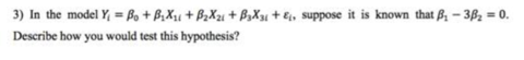
| Suppose the demand for your product is a linear function of income, relative price and the quarter of the year. Assuming the slopes are the same, explain in detail exactly how you would test the hypothesis that ceteris paribus the demand for your product is identical in the spring, summer and fall. | Include all the three dummies in the specification and forcing the coefficients of those dummies to be equal. This amounts to testing restricted versus unrestricted specifications. |
| 2) Which of the following are consequences of heteroskedasticity? a) The OLS coefficient estimates are inconsistent. b) The usual F statistic no longer has an F distribution. c) The OLS estimators are no longer BLUE. | All of them. |
| Determine the sign of the expected bias introduced by omitting a variable from the specification: In an earnings equation for workers, the impact on the coefficient of experience of omitting the variable for age. | Upward bias. Interaction of age and experience normally positive. Furthermore, age variable expected to be positive. |
| Determine the sign of the expected bias introduced by omitting a variable from the specification: In an equation for the demand for peanut butter, the impact on the coefficient of disposable income of omitting the price of peanut butter variable. | Uncertain. The coefficient of the price of peanut butter is expected to be negative as peanut butter is a normal good. Correlation between disposable income and price of peanut butter cannot be determined on this info however. |
| A friend has regressed kilograms of Brazilian coffee purchased on the real price of Brazilian coffee (PB), the real price of tea (PT), and real disposable income (Y). She found the wrong sign on PB with a t value of 0.5. She re-estimated the specification without PB and found little change in the other coefficient estimates, so she adopted the latter specification and concluded in her writeup that demand for Brazilian coffee is price inelastic. Before handing her project in she asks for your advice. What advice would you offer? | Wrong conclusion. Insignificance of the price of coffee likely caused by multicollinearity, especially in the two price variables. The variable (price of coffee) belongs in the equation. Dropping it would cause misspecification. |
| Consider a simple model to estimate the effect of personal computer (PC) ownership on grade point average for graduating students at a large university. GPA = ß(0) + ß(1)PC + (error term) where PC is binary variable indicating computer ownership. In this specification, is there reason to believe PC to be correlated with the error term? Why or why not? | PC ownership is expected to be related to parental income, as richer families can afford to buy more computers. So yes, there is expected to be correlation between PC and error term. |
| Consider a simple model to estimate the effect of personal computer (PC) ownership on grade point average for graduating students at a large university. GPA = ß(0) + ß(1)PC + (error term) where PC is binary variable indicating computer ownership. Explain why PC is likely to be related to parents’ annual income. Does this mean that parental income is a good instrumental variable (IV) for PC? Why or why not? | To serve as instrument: - Highly correlated with the variable it instruments for. - Be uncorrelated with the error term - Not be part of the original equation. Parental income does not pass these. Likely not highly correlated with PC ownership, and probably belongs in original equation (e.g. due to possibility of private tutoring). |
| What must a variable satisfy if it is to serve as an instrument in a regression? | - Highly correlated with the variable it instruments for. - Not part of the error term - Not be part of the original equation. |
| Would these independent variables violate the assumption of no perfect collinearity among independent variables? Right shoe size and left shoe size of students in your university. | Yes, it would violate the assumption of no perfect collinearity due to no difference in shoe sizes between left and right. |
| Would these independent variables violate the assumption of no perfect collinearity among independent variables? Consumption and disposable income in Denmark over 50-year period. | Although they are correlated, it would likely not violate the assumption as it is not perfectly linearly correlated. |
| Would these independent variables violate the assumption of no perfect collinearity among independent variables? Xi and 5Xi. | Yes, as these two variables are perfectly linear with each other. |
| Would these independent variables violate the assumption of no perfect collinearity among independent variables? Xi and (Xi)^3. | No, as these variables are not perfectly linear. |
| When estimating a demand function for a good where quantity demanded is a linear function of the price, you should not include an intercept because the price of the good is never zero. True, false or uncertain? Explain your reasoning. | As a rule of thumb, it is always a good idea to include the intercept. |
| Studenth = 19.6 + 0.73* Midparh; R2 = 0.45 (7.2) (0.10) where Studenth is the height of students in inches, Midparh is the average of the parental heights and the standard errors are reported in the parentheses. Interpret the estimated coefficients. What does the R2 tell you? | 19.6 = Intercept. All else being zero, the student's height would be 19.6 inches. 0.73 = by every unit average parents' height increases, the student's height will increase by 0.73 inches. The R2 of 0.45 tells us that the model only explains 45% of the difference in height among students. Thus, other variables affect height. |
| Studenth = 19.6 + 0.73* Midparh; R2 = 0.45 (7.2) (0.10) where Studenth is the height of students in inches, Midparh is the average of the parental heights and the standard errors are reported in the parentheses. If children, on average, were expected to be of the same height as their parents, then this would imply two hypotheses, one for the slope and one for the intercept. State the null hypotheses. From the info provided can you assess whether you will reject the nulls? | Slope H0: ß 1=1 Intercept H0: ß 0=0 From the standard errors, we find that both coefficients are significant as they are now. Therefore I would reject the null-hypotheses stated above, that parents and students are the same height on average. |
| In a time series setting, what is a spurious regression? Are there circumstances when it is meaningful to estimate such regressions? | Spurious regression: Situation where the co-efficients are highly significant despite them not being related to each other. When variables are co-integrated it makes sense to use such a regression. |
| Assume that religion affects educational attainment, and also affects the level of earnings conditional on education. How could I estimate the total effect of religion on earnings, and how could I estimate the marginal effect of education on earnings? What is the difference in what these terms mean? | We want to test the effect of a variable condition on another variable --> Create interaction term (religion*education) and regress on level of earnings. This is then added to the effect of religion regressed on education in order to get the total effect of religion on earnings. |
| When there are omitted variables in the regression, which are determinants of the dependent variable, then this will always bias the OLS estimator of the included variable. True, false or uncertain? Explain your reasoning. | Only true if the omitted variables are correlated with the included variables. |
| C(t) =18.5−0.07P(t) +0.93YD(t) −0.74D1(t) −1.3D2(t) −1.3D3(t) Ct is per-capita pounds of pork consumed in the United States in quarter t Pt is the price of a hundred pounds of pork (in dollars) in quarter t YDt is per capita disposable income (in dollars) in quarter t D1t is a dummy equal to 1 in the first quarter (Jan.–Mar.) of the year and 0 otherwise D2t is a dummy equal to 1 in the second quarter of the year and 0 otherwise D3t is a dummy equal to 1 in the third quarter of the year and 0 otherwise (a) What is the meaning of the estimated coefficient of YD? | Disposable income is positively correlated to the pork consumption. An extra dollar of disposable income will lead to a 0.93 pound increase in pork consumption – all else being equal. |
| C(t) =18.5−0.07P(t) +0.93YD(t) −0.74D1(t) −1.3D2(t) −1.3D3(t) Ct is per-capita pounds of pork consumed in the United States in quarter t Pt is the price of a hundred pounds of pork (in dollars) in quarter t YDt is per capita disposable income (in dollars) in quarter t D1t is a dummy equal to 1 in the first quarter (Jan.–Mar.) of the year and 0 otherwise D2t is a dummy equal to 1 in the second quarter of the year and 0 otherwise D3t is a dummy equal to 1 in the third quarter of the year and 0 otherwise Specify expected signs for each of the coefficients. Explain your reasoning | The price is expected to be negatively correlated, since the higher the price, the less consumption. Disposable income expected to be positive. Cannot state expected sign of seasons without more information. |
| Wi = -11,4 + 0,31Ai – 0,003Ai^2 + 1,02Si + 1,23Ui (2,98) (1,49) (5,04) (1,21) N = 34; Adjusted R2 = 0,14 Wi = the hourly wage (in Euros) of the ith worker Ai = the age of the ith worker Si = the number of years of education of the ith worker Ui = a dummy variable equal to 1 if the ith worker is a union member, 0 otherwise What is the meaning of including A2 in the equation? What relationship between A and W do the signs of the coefficients imply? Why doesn’t the inclusion of A and A2 violate the assumption of no perfect collinearity between two independent variables? | The rationale behind the inclusion of the quadratic term for age is the curve linear relationship between wage and age. The sign of the coefficients suggest an inverted U-shaped relationship (That is, older workers earn more per hour, probably due to increase in experience, but after a certain age further increases in age lead to lower hourly wage). Does not violate perfect collinearity condition since they are not perfectly linear. |
| Wi = -11,4 + 0,31Ai – 0,003Ai^2 + 1,02Si + 1,23Ui (2,98) (1,49) (5,04) (1,21) N = 34; Adjusted R2 = 0,14 Wi = the hourly wage (in Euros) of the ith worker Ai = the age of the ith worker Si = the number of years of education of the ith worker Ui = a dummy variable equal to 1 if the ith worker is a union member, 0 otherwise Even though you have been told not to focus on the value of the intercept, isn’t -11,4 too low to just ignore? What should be done to correct this problem? | Magnitude of intercept impacted by missing variables. Currently looks as if a person who is not a union member, zero years of experience, and zero years old will have a negative hourly wage. Such an individual does not exist. One solution: Make the average age (mean) of the sample zero. Thus the intercept is a non-union member, zero years of experience, and the average age of the sample. |
| Wi = -11,4 + 0,31Ai – 0,003Ai^2 + 1,02Si + 1,23Ui (2,98) (1,49) (5,04) (1,21) N = 34; Adjusted R2 = 0,14 Wi = the hourly wage (in Euros) of the ith worker Ai = the age of the ith worker Si = the number of years of education of the ith worker Ui = a dummy variable equal to 1 if the ith worker is a union member, 0 otherwise Would your boss be happy with your regression results? Can you conclude that union membership improves workers’ well-being? Why or why not? | Boss would not be happy. - Co-efficient of union dummy not significant (should be over 2) - R2 is very low suggesting omitted variable bias - Sample size is very small |
| Suppose I estimate an OLS regression of the time series variable Y(t) on X(t) and find strong evidence that the residuals are serially correlated. Does this imply my coefficient estimates are inconsistent? | No. Serial correlation does not affect unbiasedness or consistency of coefficient estimators. Only affects efficiency. Positive serial correlation --> Smaller standard errors than they really are, thus the (wrong) conclusion that the results are more precise than they really are. |
| You need to impose the restriction into the original equation, estimate the new equation it with OLS and perform an F-test of restricted versus un-restricted models. | |
| Suppose you compute a sample statistic q to estimate a population quantity Q. If q is an unbiased estimator of Q, then q = Q. True, false or uncertain. Explain your reasoning carefully. | False. The actual sample statistic, q, that we calculate is just a random draw from that sampling distribution, which may or may not be equal to its mean, Q. For it to be unbiased: q must be centered around Q. |
| In the presence of heteroskedasticity coefficient estimates from a logistic regression are biased and inconsistent. True, false or uncertain? Explain your reasoning. | True. In logistic regression, heteroskedasticity leads to bias and inconsistent estimates. In OLS, it doesn't affect bias, but only efficiency. |
| Omitting a relevant explanatory variable that is uncorrelated with the other independent variables causes bias and a decrease in standard errors. True, false or uncertain? Explain your reasoning. | Both true and false. Since it is uncorrelated, it does not affect the bias. Omitting the variable however, likely increases precision due to higher degrees of freedom --> Lower standard errors. |
| Imagine you estimate a model where earnings is a function of a bunch of independent variables that are inter-related (they cause each other), and nothing in the model is statistically significant. Does that mean that these independent variables do not influence earnings? If you believed that they really did influence earnings, what might you do? | Could be a sign of multicollinearity. Next steps: Explore bivariate correlations and VIFs. If detection of multicollinearity --> Find a way to re-define the variables or find a way to combine them so that it makes sense. |
| C(t) =18.5−0.07P(t) +0.93YD(t) −0.74D(1)(t) −1.3D(2)(t) −1.3D(3)(t) C(t) = per-capita pounds of pork consumed in the United States in quarter t P(t) = the price of a hundred pounds of pork (in dollars) in quarter t YD(t) = per capita disposable income (in dollars) in quarter t D(1)(t) = dummy equal to 1 in the first quarter (Jan.–Mar.) of the year and 0 otherwise D(2)(t) = dummy equal to 1 in the second quarter of the year and 0 otherwise D(3)(t) = dummy equal to 1 in the third quarter of the year and 0 otherwise What is the meaning of the estimated coefficient of YD? | It is the marginal effect of an increase in income on consumption of pork. |
| C(t) =18.5−0.07P(t) +0.93YD(t) −0.74D(1)(t) −1.3D(2)(t) −1.3D(3)(t) C(t) = per-capita pounds of pork consumed in the United States in quarter t P(t) = the price of a hundred pounds of pork (in dollars) in quarter t YD(t) = per capita disposable income (in dollars) in quarter t D(1)(t) = dummy equal to 1 in the first quarter (Jan.–Mar.) of the year and 0 otherwise D(2)(t) = dummy equal to 1 in the second quarter of the year and 0 otherwise D(3)(t) = dummy equal to 1 in the third quarter of the year and 0 otherwise Suppose we changed the definition of D(3)(t) so that it was equal to 1 in the fourth quarter and 0 otherwise and re-estimated the equation with all the other variables unchanged. Which of the estimated coefficients would change? | The coefficients of the dummies will change because the reference quarter is different. The rest of coefficients should not change. |
| Briefly explain the meaning of the following terms: • A time series integrated of order 2 • Stochastic error term • Endogenous variable • Unobserved heterogeneity | - Time series integrated of order 2: ??? - Stochastic error term: Term added to regression equation to introduce all of the variation that cannot be explained by the x's. - Endogenous variable: Variable that is influenced or determined by another variable in the model. - Unobserved heterogeneity: variation/differences among cases which are not measured |
| A:Y = 125.0−15.0X1 −1.0X2 +1.5X3 R2 = 0.75 B:Y = 123.0−14.0X1 +5.5X2 −3.7X4 R2 = 0.73 Where Y = the number of joggers on a given day, X1 = inches of rain that day, X2 = hours of sunshine that day, X3 = the high temperature for that day (in Celcius), and X4 = the number of classes with term papers due the next day. Which of the two (admittedly hypothetical) equations do your prefer and why? | Prefer B as the coefficients have the expected signs. |
| A:Y = 125.0−15.0X1 −1.0X2 +1.5X3 R2 = 0.75 B:Y = 123.0−14.0X1 +5.5X2 −3.7X3 R2 = 0.73 Where Y = the number of joggers on a given day, X1 = inches of rain that day, X2 = hours of sunshine that day, X3 = the high temperature for that day (in Celcius), and X4 = the number of classes with term papers due the next day. How is it possible to get different estimate signs for the coefficient of the same variable using the same data? | It is possible to get different signs for the coefficient of the same variable because although we are using the same data we are estimating different specifications, ie., variables in the two specifications are not exactly the same. The sign flip is a sign of multicollinearity in one of the specifications. When two variables are highly collinear, removing one from the specification leads to sign flip of the other. |
| Carefully outline (be brief!) a description of the problem typically referred to as pure heteroskedasticity. (a) What is it? (b) What are its consequences? (c) How do you diagnose it? (d) What do you do to get rid of it? | Pure heteroskedasticity refers to the situation when the variance of the error term is not constant for all observations. Coefficients are unbiased, but standard errors are inconsistent. We cannot rely on t and F tests. We test for heteroskedasticity through generic tests or more specific tests if we suspect it is driven by a given variable. Often, the composition of the sample will tell us that data is heteroskedastic. To account for it, we can apply the robust correction or WLS. |
| Suppose I estimate an OLS regression of the time series variable Yt on Xt and find strong evidence that the residuals are serially correlated. Does this imply my coefficient estimates are inconsistent? | Coefficients are unbiased but standard errors are inconsistent, making the t and F test unreliable. |
| What examples are there of data reduction techniques? Purpose of data reduction? | Simple tabulation, principal component analysis, factor analysis, cluster analysis. Obtain a reduced representation of the data set that is much smaller in volume but yet produces the same (or almost the same) analytical results |
| Main issue of cluster analysis. | Cluster analysis has no mechanism for differentiating between relevant and irrelevant variables. |
| When is non-parametric statistics used? | - When data is nominal - When data is ordinal - When no assumptions about the population distribution can be made |
| In an OLS regression, what does BLUE stand for? | Best Linear Unbiased Estimator. |
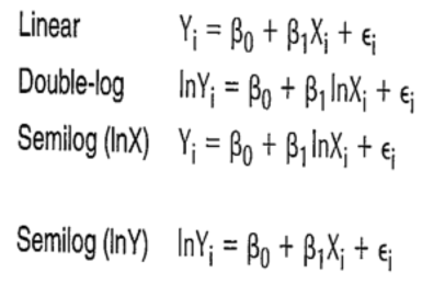
| Interpret ß(1) in each of the equations. | Interpretation of ß(1): Linear: Slope of Y Double-log: Elasticity of Y Semilog: unit change in y with regards to 1 percentage increase in X Semilog (lnY): Percentage increase with regards to 1 unit increase in X. |
| Describe omitted variable issue. - What is it? - What are the consequences? - How can it be detected? - How can it be corrected? | - Omittance of a relevant variable. - Bias in the coefficients. - Theory, unexpected signs, surprisingly poor fits. - By including the omitted variable or proxy. |
| What reason is there to include quadratic terms in regressions? | To account for non-linear relationships. |
| - When testing for multicollinearity through VIFs, what value should not be exceeded? - What value should not be exceeded when looking at bivariate coefficient of correlation in Stata? What is the command? | - 5. - 0,8 should not be exceeded. Command is corr. |
| For the residuals to have a normal distribution, what value must the coefficient of skewness lie in between? | (-1;1) |
| What value should a t-statistic be in order to reject the null? | Above 2. |
| When do you use logit/probit models? | When the dependent variable is binary/dichotomous. |
| Difference in cluster and factor analysis | Cluster: Distance/proximity Factor: Covariance |
Want to create your own Flashcards for free with GoConqr? Learn more.